Simulated data

The boa data is simulated using different Gaussian mixtures with varied centres and weights (see section format for the simulation code). Theses data are simulated for demonstrating the usage of four diagnostic plots in the package, users can create their own guided tour data objects and diagnose with the visualisation designed in this package.

holes_1d_geo

holes_1d_better

holes_2d_better

holes_2d_better_max_tries

boa

boa5

boa6

Format

The code for simulating each data object is as follows:

set.seed(123456);
holes_1d_geo <-
  animate_dist(boa5, tour_path = guided_tour(holes(), d = 1,
                                             search_f =  search_geodesic),
               rescale = FALSE)

set.seed(123456)
holes_1d_better <-
  animate_dist(boa5, tour_path = guided_tour(holes(), d = 1,
                                             search_f =  search_better),
               rescale = FALSE)


set.seed(123456)
holes_2d_better <-
  animate_xy(boa6, tour_path = guided_tour(holes(), d = 2,
                                           search_f =  search_better),
            rescale = FALSE)

set.seed(123456)
holes_2d_better_max_tries <-
  animate_xy(boa6, tour_path = guided_tour(holes(), d = 2,
                                           search_f = search_better,
                                           max.tries = 500),
             rescale = FALSE)

library(tidyverse)
set.seed(1234)
x1 <- rnorm(1000, 0, 1)
x2 <- sample(c(rnorm(500, -3, 1), rnorm(500, 3, 1)), size = 1000)
x3 <- sample(c(rep(-1, 500), rep(1, 500)), size = 1000)
x4 <- sample(c(rnorm(250, -3, 1), rnorm(750, 3, 1)), size = 1000)
x5 <- sample(c(rnorm(330, -5, 1), rnorm(340, 0, 1), rnorm(330, 5, 1)), size = 1000)
x6 <- sample(c(rnorm(450, -5, 1), rnorm(100, 0, 1), rnorm(450, 5, 1)), size = 1000)
x7 <- sample(c(rnorm(500, -5, 1), rnorm(500, 5, 1)), size = 1000)
x8 <- rnorm(1000, 0, 1)
x9 <- rnorm(1000, 0, 1)
x10 <- rnorm(1000, 0, 1)

boa <- tibble(x1 = x1, x2 = x2, x3 = x3, x4 = x4, x5 = x5,
              x6 = x6, x7 = x7, x8 = x8, x9 = x9, x10 = x10) 
boa <- as_tibble(scale(boa))
boa5 <- select(boa, x1, x2, x8: x10)
boa6 <- select(boa, x1, x2, x7: x10)

An object of class tbl_df (inherits from tbl, data.frame) with 79 rows and 8 columns.

An object of class tbl_df (inherits from tbl, data.frame) with 98 rows and 8 columns.

An object of class tbl_df (inherits from tbl, data.frame) with 1499 rows and 8 columns.

An object of class tbl_df (inherits from tbl, data.frame) with 1000 rows and 10 columns.

An object of class tbl_df (inherits from tbl, data.frame) with 1000 rows and 5 columns.

An object of class tbl_df (inherits from tbl, data.frame) with 1000 rows and 6 columns.

Details

The prefix holes_* indicates the use of holes index in the guided tour. The suffix *_better/geo indicates the optimiser used: search_better and search_geodesic.

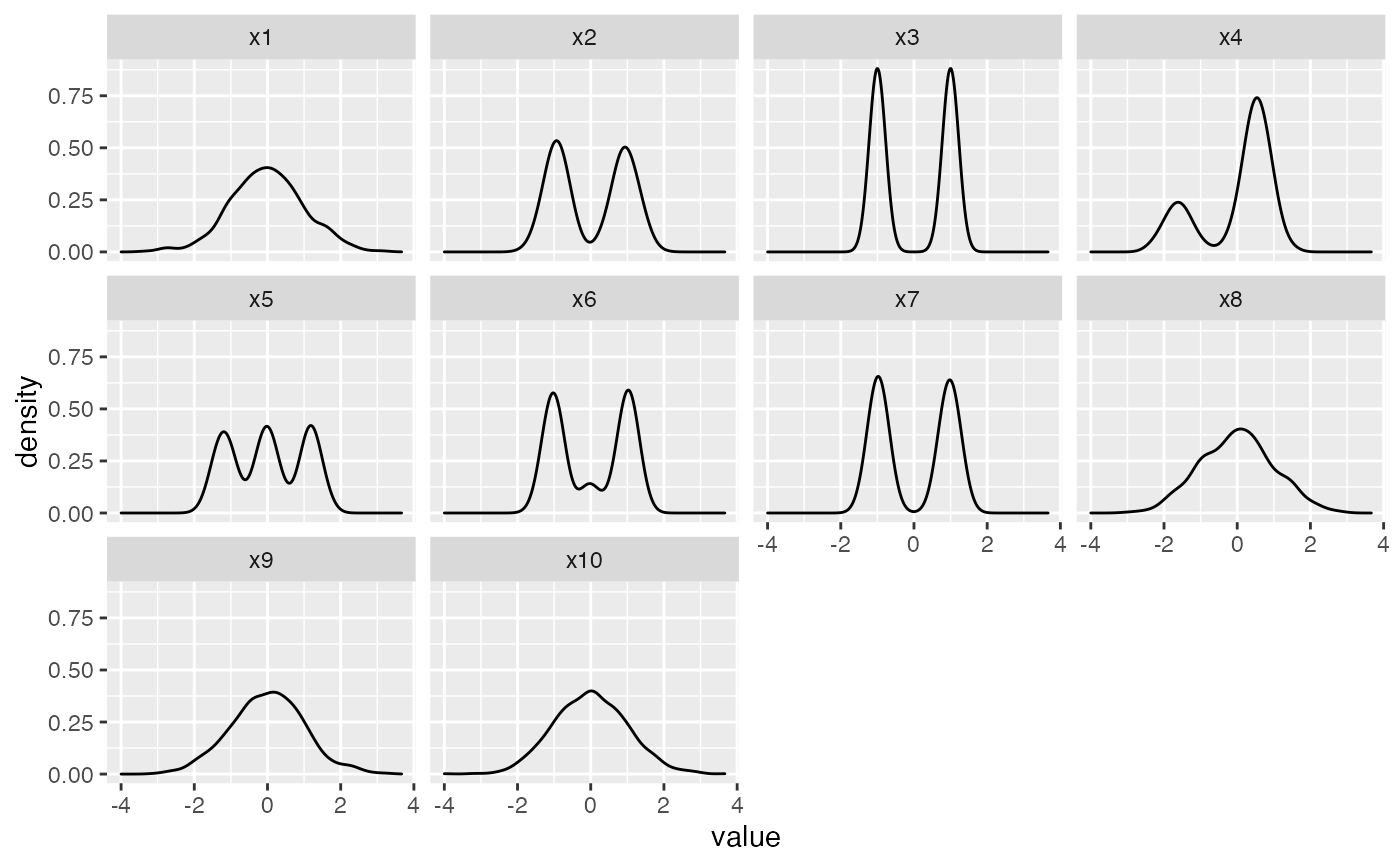
The name boa comes from the fact that the density plot of each variable in the data looks like boa constrictors swallowing multiple French baguettes, rather than elephants, as in the novella the little prince.

Examples

library(ggplot2)
library(tidyr)
library(dplyr)
#> 
#> Attaching package: ‘dplyr’
#> The following objects are masked from ‘package:stats’:
#> 
#>     filter, lag
#> The following objects are masked from ‘package:base’:
#> 
#>     intersect, setdiff, setequal, union
boa %>%
  pivot_longer(cols = x1:x10, names_to = "var", values_to = "value") %>%
  mutate(var = forcats::fct_relevel(as.factor(var), paste0("x", 1:10))) %>%
  ggplot(aes(x = value)) +
  geom_density() +
  facet_wrap(vars(var))