Elements of Data Science
SDS 322E

H. Sherry Zhang
Department of Statistics and Data Sciences
The University of Texas at Austin

Fall 2025

Learning objectives

• Understand the concept of tidy data: identify whether a dataset is tidy or not (we will cover how to tidy a messy data in code in week 4).

• Understand the pipe operator (|>): you need to know how to read and think about code with pipes.

Seek helps during the office hours

GDC (Gates Dell Complex) level 7 open space

• Monday 10-12pm after class with me
• Tuesday 2-3:15pm with Luke Bellinger (UGCA)
• Wednesday 3-5pm with Arka Sinha (Grad TA)
• Friday 10-11am with Luke Bellinger (UGCA)

Tidy data

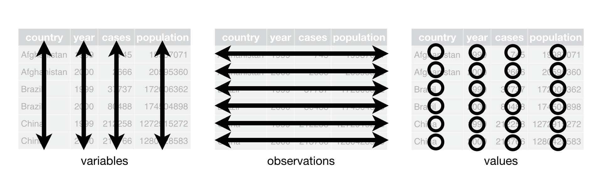
• Each variable is a column
• Each observation is a row
• Each cell is a single value

Is this tidy? (1/8)

income and religion in the US produced by Pew Research Center in 2014

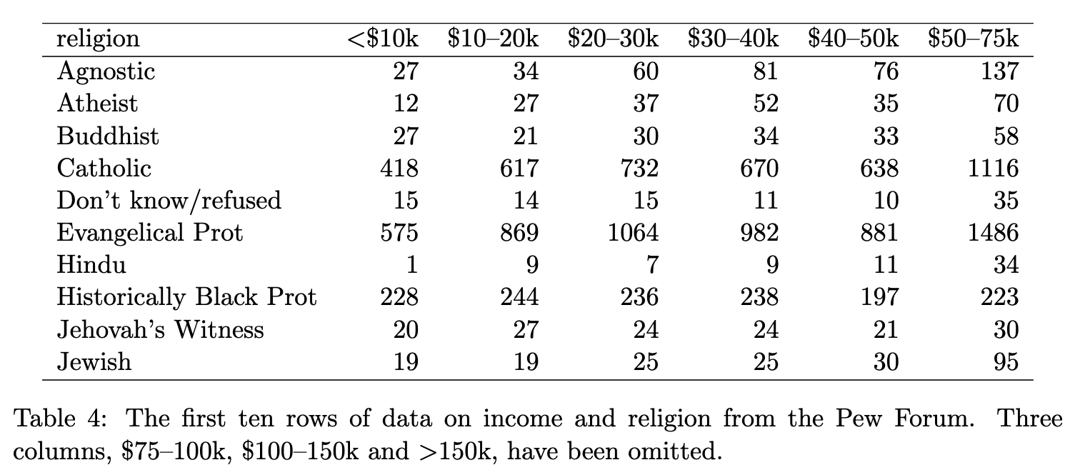
❌ No, because values (<$10k, $10-20k, $20-30k, …) are in variable names

Is this tidy? (2/8)

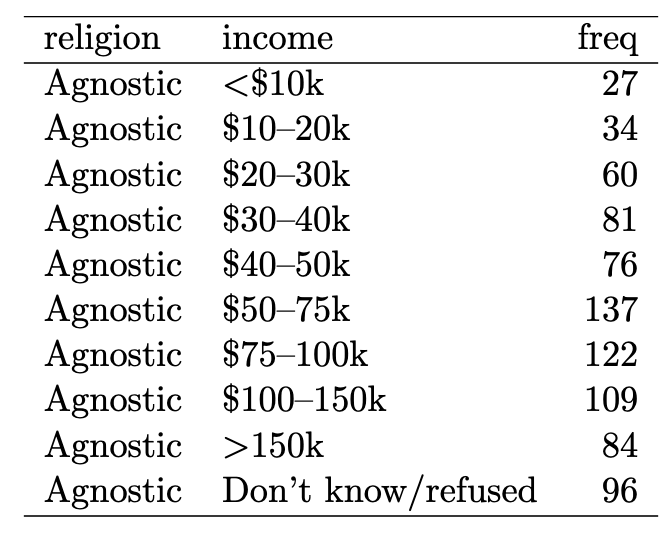
✅ Yes, because 1) The variables are: religion, income, and freq (count), 2) The observation is a demographic unit corresponding to a combination of religion and income

Is this tidy? (3/8)

The Billboard dataset: the date a song first entered the Billboard Top 100

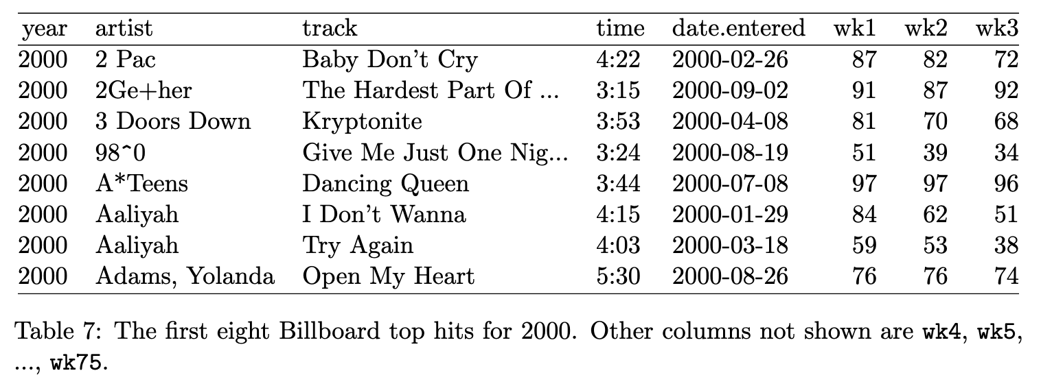
❌: No, because wk1, wk2, … are values, not variables - they should be recorded in cells rather than in column names

Is this tidy? (4/8)

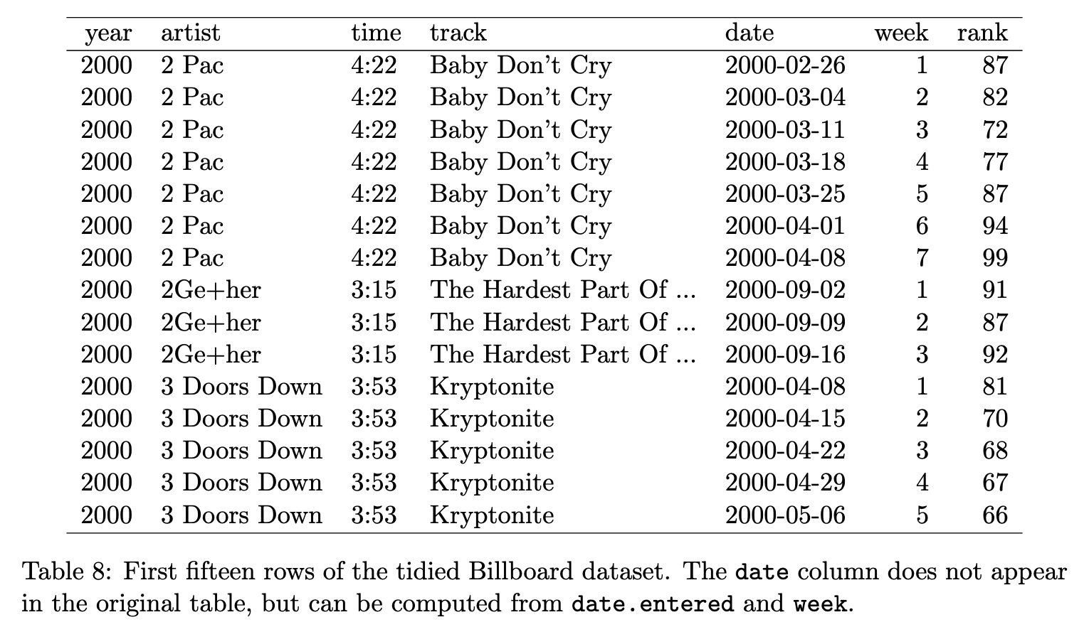
✅ Yes, because 1) The variables are: year, artist, time, track, date, week, and rank, 2) The observation is a recorded rank of a song in a particular week

Is this tidy? (5/8)

Number of cases of TB (tuberculosis)

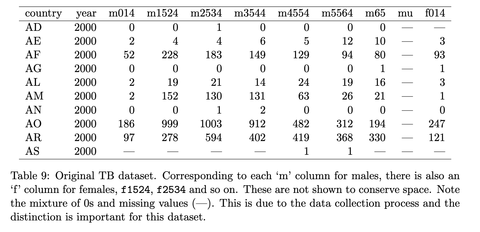
Some information: m014 means for male, 1-14 year old, m1524 means for male 15-24 year old, etc.

❌ No, because the column names contain multiple variable names: gender (m/f) and age (both lower end and higher end of the range).

Is this tidy? (6/8)

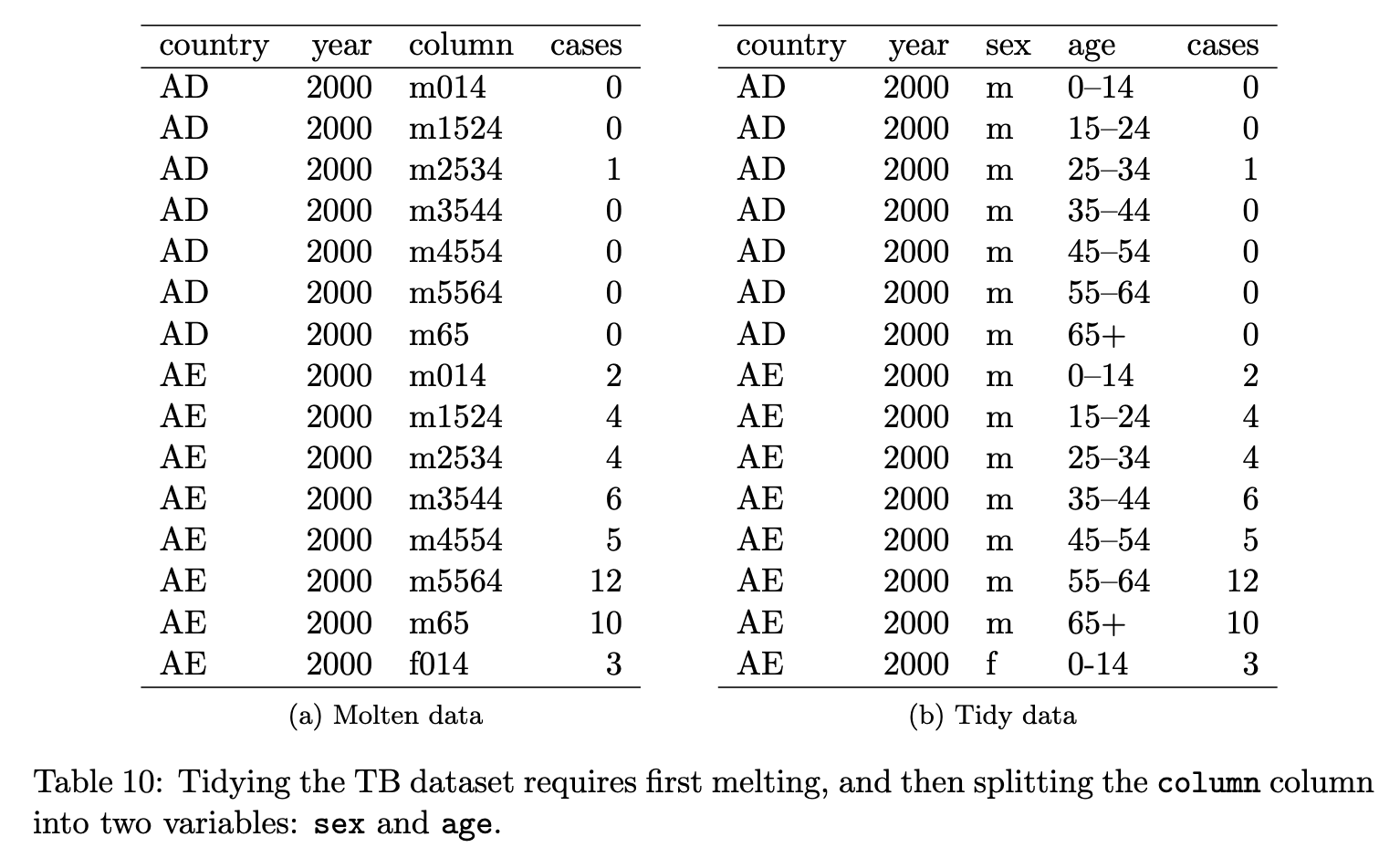
✅ Yes, because 1) The variables are: country, year, column, and cases, and 2) the observation is the number of cases per year, per gender age group, per country

Both are tidy data - you will learn in week 4 how to clean it from (a) to (b)

Is this tidy? (7/8) - the gapminder data

gapminder::gapminder

# A tibble: 1,704 × 6
   country     continent  year lifeExp      pop gdpPercap
   <fct>       <fct>     <int>   <dbl>    <int>     <dbl>
 1 Afghanistan Asia       1952    28.8  8425333      779.
 2 Afghanistan Asia       1957    30.3  9240934      821.
 3 Afghanistan Asia       1962    32.0 10267083      853.
 4 Afghanistan Asia       1967    34.0 11537966      836.
 5 Afghanistan Asia       1972    36.1 13079460      740.
 6 Afghanistan Asia       1977    38.4 14880372      786.
 7 Afghanistan Asia       1982    39.9 12881816      978.
 8 Afghanistan Asia       1987    40.8 13867957      852.
 9 Afghanistan Asia       1992    41.7 16317921      649.
10 Afghanistan Asia       1997    41.8 22227415      635.
# ℹ 1,694 more rows

✅ Yes, because

• Each variable forms a column: country, continent, year, lifeExp, pop, gdpPercap

• Each observation forms a row: each row is a country in a particular year

• Each value forms a cell: e.g. life expectancy of Afghanistan in 1952 is 28.801

Is this tidy? (8/8) - the flight data

nycflights13::flights

# A tibble: 336,776 × 19
    year month   day dep_time sched_dep_time dep_delay arr_time
   <int> <int> <int>    <int>          <int>     <dbl>    <int>
 1  2013     1     1      517            515         2      830
 2  2013     1     1      533            529         4      850
 3  2013     1     1      542            540         2      923
 4  2013     1     1      544            545        -1     1004
 5  2013     1     1      554            600        -6      812
 6  2013     1     1      554            558        -4      740
 7  2013     1     1      555            600        -5      913
 8  2013     1     1      557            600        -3      709
 9  2013     1     1      557            600        -3      838
10  2013     1     1      558            600        -2      753
# ℹ 336,766 more rows
# ℹ 12 more variables: sched_arr_time <int>, arr_delay <dbl>,
#   carrier <chr>, flight <int>, tailnum <chr>, origin <chr>,
#   dest <chr>, air_time <dbl>, distance <dbl>, hour <dbl>,
#   minute <dbl>, time_hour <dttm>

✅ Yes, because 1) each variable forms a column, 2) each observation forms a row: each row is one flight, and 3) each value forms a cell

The pipe operator

If you download the Friday code, you will see something like this:

gapminder$country |> unique() |> length()

Once upon a time

Abstraction	Example
FUN_1(DATA)	unique(gapminder$lifeExp)
FUN_2(FUN_1(DATA))	length(unique(gapminder$lifeExp))

Abstraction: FUN_1(DATA, arg1 = val1, arg2 = val2)

Example: mutate(mtcars, kpl = mpg * 0.425)

Abstraction: FUN_2(FUN_1(DATA, arg1 = val1, arg2 = val2), arg3 = val3)

Example: filter(mutate(mtcars, kpl = mpg * 0.425), vs ==0)

Abstraction: FUN_3(FUN_2(FUN_1(DATA, arg1 = val1, arg2 = val2), arg3 = val3), arg4 = val4)

Example: group_by(filter(mutate(mtcars, kpl = mpg * 0.425), vs ==0), cyl)

We could keep going on to make the code annoyingly long . . .

Abstraction: FUN_4(FUN_3(FUN_2(FUN_1(DATA, arg1 = val1, arg2 = val2), arg3 = val3), arg4 = val4), arg5 = val5)

Example: summarize(group_by(filter(mutate(mtcars, kpl = mpg * 0.425), vs ==0), cyl), disp = mean(disp, na.rm = TRUE), kpl = mean(kpl, na.rm = TRUE))|

With line breaks we can do:

summarize(
  group_by(
    filter(
      mutate(
        mtcars, 
        kpl = mpg * 0.425), 
      vs ==0), 
    cyl), 
  disp = mean(disp, na.rm = TRUE), 
  kpl = mean(kpl, na.rm = TRUE)
  )

We need to read from middle out 😿

How about this?

mtcars |>
  mutate(kpl = mpg * 0.425144) |>
  filter(vs == 0) |>
  group_by(cyl) |>
  summarize(
    disp = mean(disp, na.rm = TRUE),
    kpl = mean(kpl, na.rm = TRUE)
    )

Much more natural 😄

Why this works?

The pipe operator abstracts out the first argument of a function, so

unique(gapminder$country) is equivalent to gapminder$country |> unique()

This is a powerful abstraction that allows us to chain together a sequence of data transformations (aka dplyr functions) in a clear and readable way since all the tidyverse functions take the data frame as the first argument.

• mtcars is a data frame
• mutate() is a function that takes the dataset as its first argument, so we can do mtcars |> mutate(kpl = mpg * 0.425144)

• The output of above is still a data frame, so we can pipe it to the next function filter():

mtcars |> mutate(kpl = mpg * 0.425144) |> filter(vs == 0)

Why this works?

• The output of this is still a data frame, so we can pipe it to the next function group_by():

mtcars |> 
  mutate(kpl = mpg * 0.425144) |> 
  filter(vs == 0) |> 
  group_by(cyl)

• The output of this is still a data frame, so we can pipe it to the next function summarize():

mtcars |> 
  mutate(kpl = mpg * 0.425144) |> 
  filter(vs == 0) |> 
  group_by(cyl) |> 
  summarize(disp = mean(disp, na.rm = TRUE),
            kpl = mean(kpl, na.rm = TRUE))

Pipe logistics

On your keyboard, the pipe operator is produced by:

• | (vertical bar): shift + \ (backslash), plus
• > (greater than): shift + . (period).

There is a shortcut: control + shift + M (for Mac: command + shift + M)

You will see a lot of pipes in the Friday class - be prepared!

Now, practice last Friday’s script via

usethis::create_from_github("SDS322E-2025FALL/0103-basics", fork = FALSE)