# A tibble: 99,338 × 6
    long   lat group order region subregion
   <dbl> <dbl> <dbl> <int> <chr>  <chr>
 1 -69.9  12.5     1     1 Aruba  <NA>
 2 -69.9  12.4     1     2 Aruba  <NA>
 3 -69.9  12.4     1     3 Aruba  <NA>
 4 -70.0  12.5     1     4 Aruba  <NA>
 5 -70.1  12.5     1     5 Aruba  <NA>
 6 -70.1  12.6     1     6 Aruba  <NA>
 7 -70.0  12.6     1     7 Aruba  <NA>
 8 -70.0  12.6     1     8 Aruba  <NA>
 9 -69.9  12.5     1     9 Aruba  <NA>
10 -69.9  12.5     1    10 Aruba  <NA>
# ℹ 99,328 more rowsElements of Data Science
SDS 322E
Make a basic map
Make it prettier

Make it prettier

Make it prettier
Spatial data science
Spatial data science is actually worth a whole course (or more) on its own.
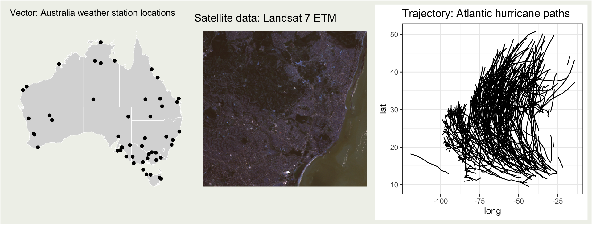
The geometry column
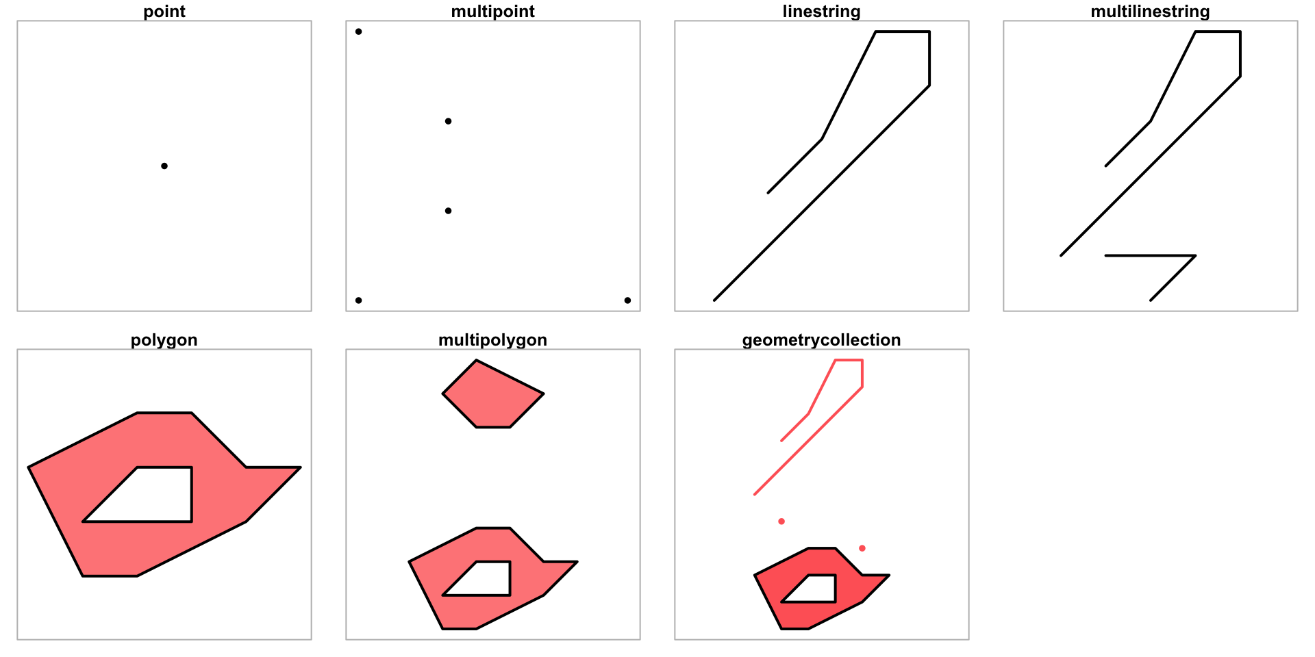
point, linestring and polygon are the most common geometries.
Coordinate Reference System (CRS)
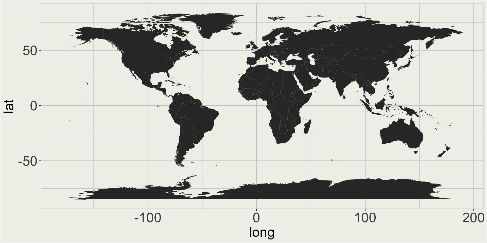
Have you ever wondered how do we show the 3D globe on a 2D map?
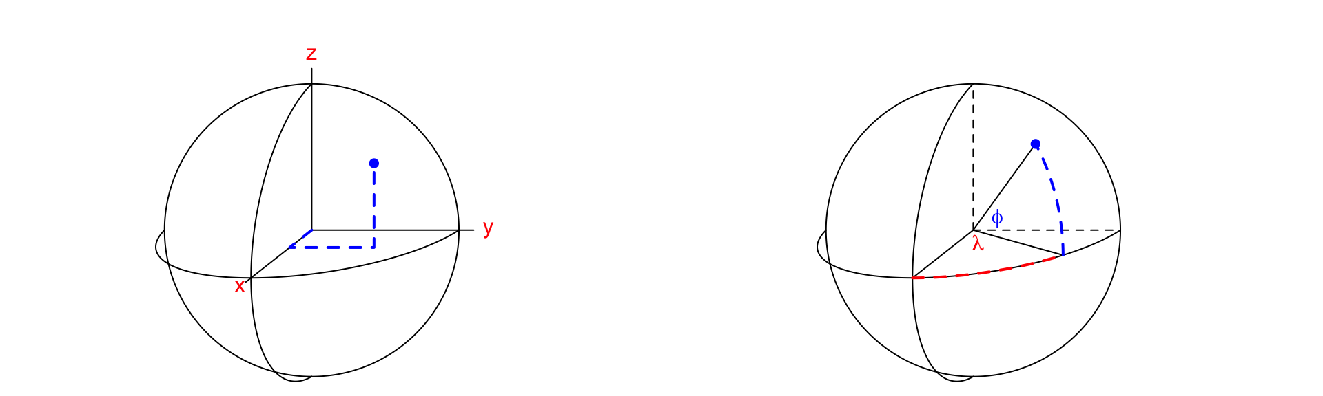
- The longitude and latitude coordinates are angles: (\(\lambda\), \(\phi\))
- We could use some complicated formula to translate these angles into distances on a flat map - map projects
There are many different map projections
Common CRSs include WGS84 (EPSG:4326) and Web Mercator (EPSG:3857) for global maps
WGS84 (EPSG:4326)
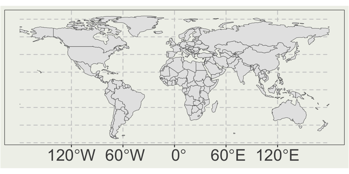
To change the CRS of an sf object, use st_transform(). To get the current CRS, use st_crs().
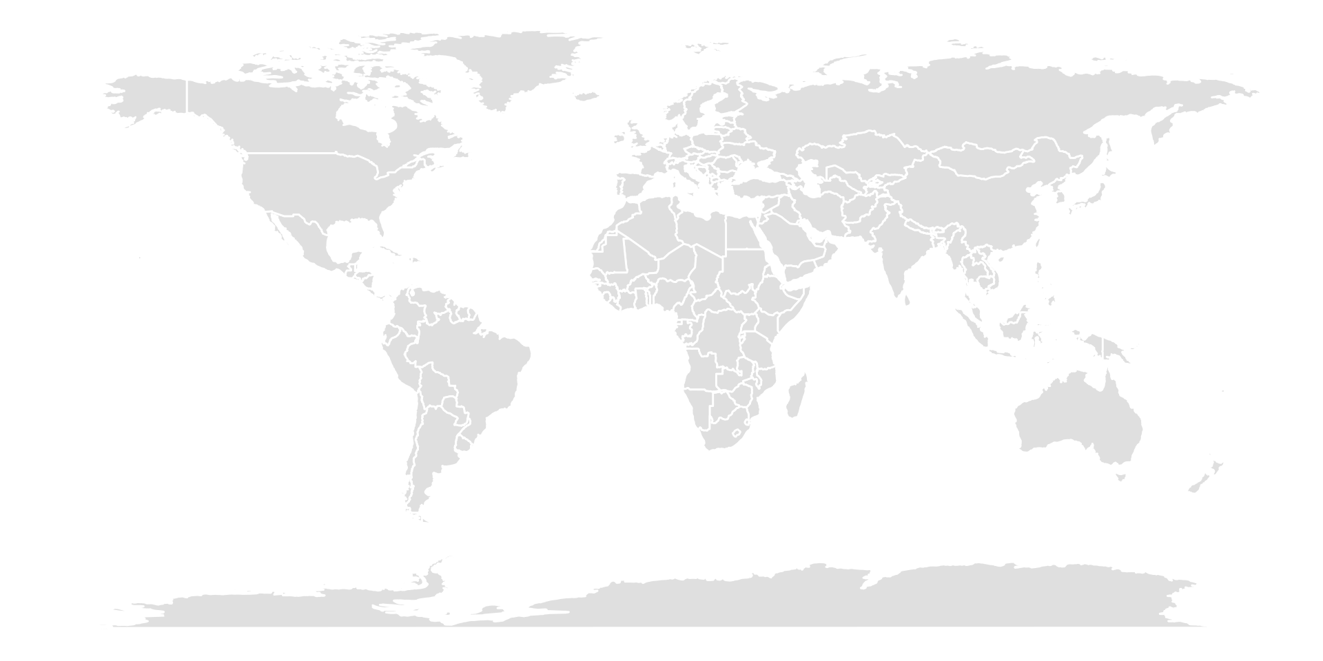
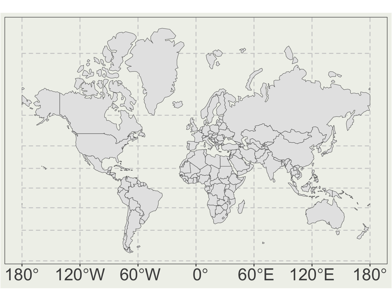
Web Mercator (EPSG:3857)
For specific regions, use a local projection
NAD27 / US National Atlas Equal Area
Simple feature collection with 51 features and 3 fields
Geometry type: MULTIPOLYGON
Dimension:     XY
Bounding box:  xmin: -2584074 ymin: -2602555 xmax: 2516258 ymax: 731628.1
Projected CRS: NAD27 / US National Atlas Equal Area
First 10 features:
   fips abbr                 full                           geom
1    02   AK               Alaska MULTIPOLYGON (((-2390688 -2...
2    01   AL              Alabama MULTIPOLYGON (((1091785 -13...
3    05   AR             Arkansas MULTIPOLYGON (((482022.2 -9...
4    04   AZ              Arizona MULTIPOLYGON (((-1386064 -1...
5    06   CA           California MULTIPOLYGON (((-1716581 -1...
6    08   CO             Colorado MULTIPOLYGON (((-787705.6 -...
7    09   CT          Connecticut MULTIPOLYGON (((2156162 -83...
8    11   DC District of Columbia MULTIPOLYGON (((1950799 -40...
9    10   DE             Delaware MULTIPOLYGON (((2037480 -28...
10   12   FL              Florida MULTIPOLYGON (((1853163 -20...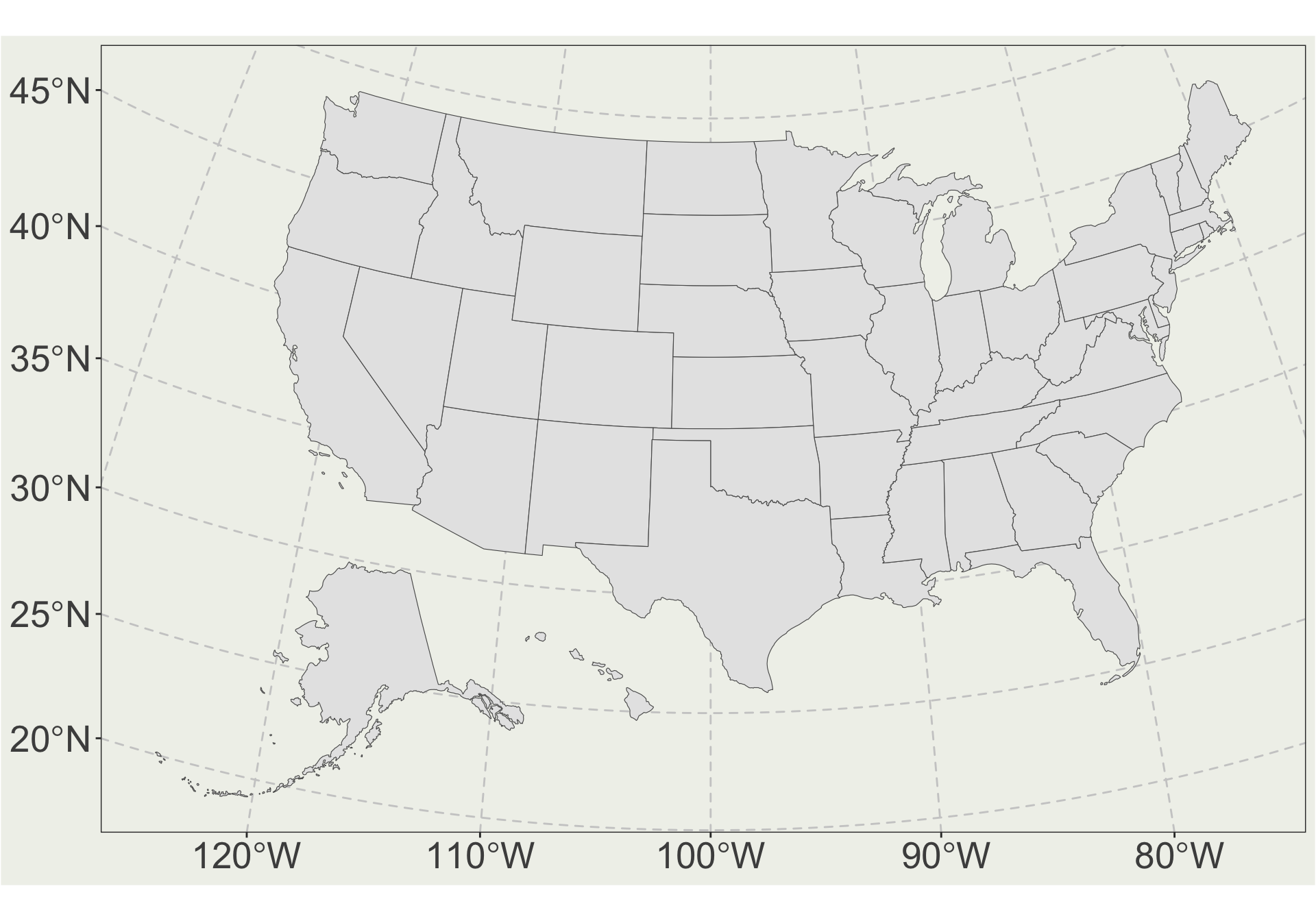
Spatial operators
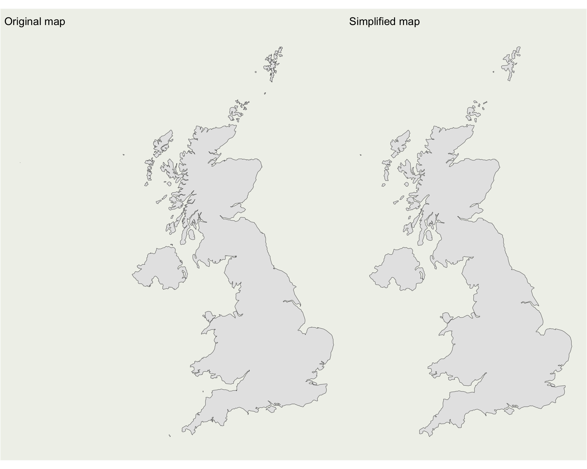
Large spatial data can be slow to render. Simplifying the geometry can help: rmapshaper::ms_simplify()
Get a google map background: the ggmap package
You will need to get a Google API key for this: ?ggmap::register_google()
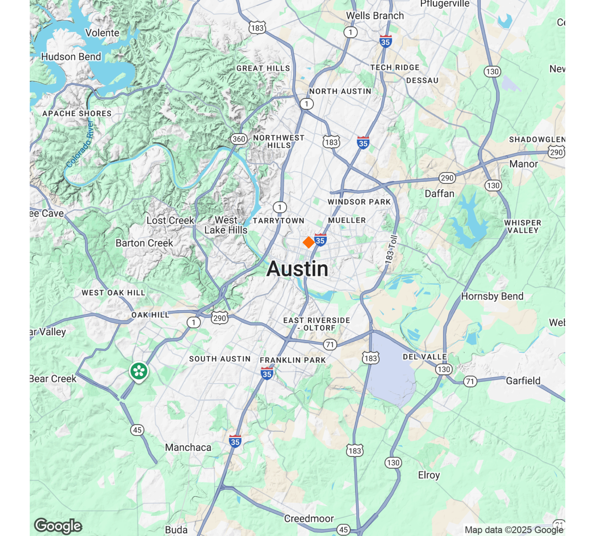
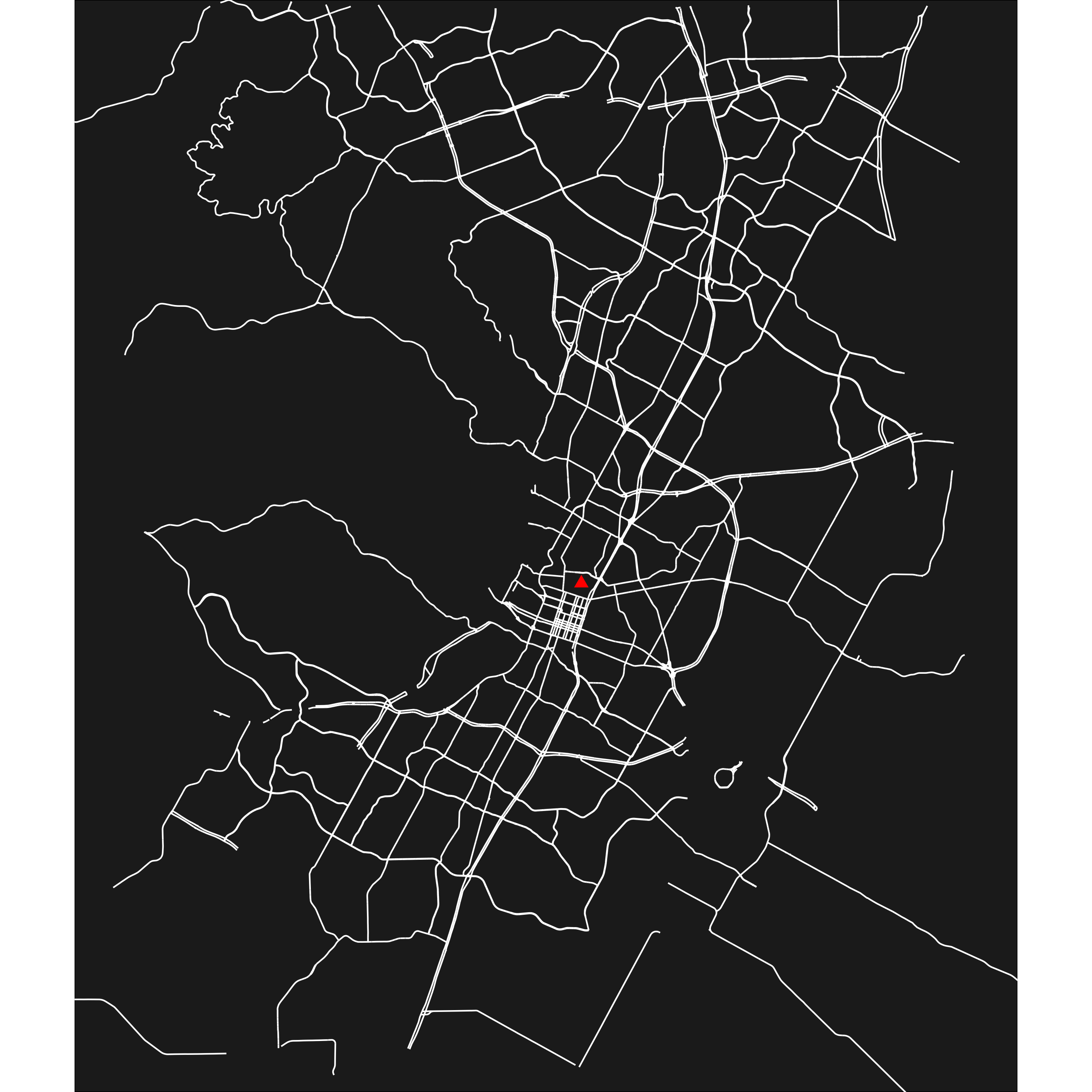
Let’s play
We can also find online the coordinates for UT and plot them together
UT <- tibble(x = -97.7335, y = 30.2850) |>
  sf::st_as_sf(coords = c("x", "y"), crs = 4326)

ggplot() +
  geom_sf(data = aus_highway, color = "white") +
  geom_sf(data = UT, color = "red",
          size = 3, shape = 17) +
  coord_sf(xlim = c(-97.95, -97.55),
           ylim = c(30.1, 30.5)) +
  theme_void() +
  theme(
    panel.background = element_rect(fill = "grey10"),
    panel.grid = element_blank()
    )
You can change the location to your favorite city and explore more features in Open Street Map!