Elements of Data Science
SDS 322E

H. Sherry Zhang
Department of Statistics and Data Sciences
The University of Texas at Austin

Fall 2025

Learning objectives

• Master the pivot_longer() and pivot_wider() functions in the tidyr package
  • Refresh on the concept of tidy data
  • Understand when and how to use pivot_longer() and pivot_wider()
• Practice combining pivot_longer() and pivot_wider() with other tidyr functions such as separate()
• Apply data wrangling skills to prepare data for visualization (the anscombe example)

Tidy data

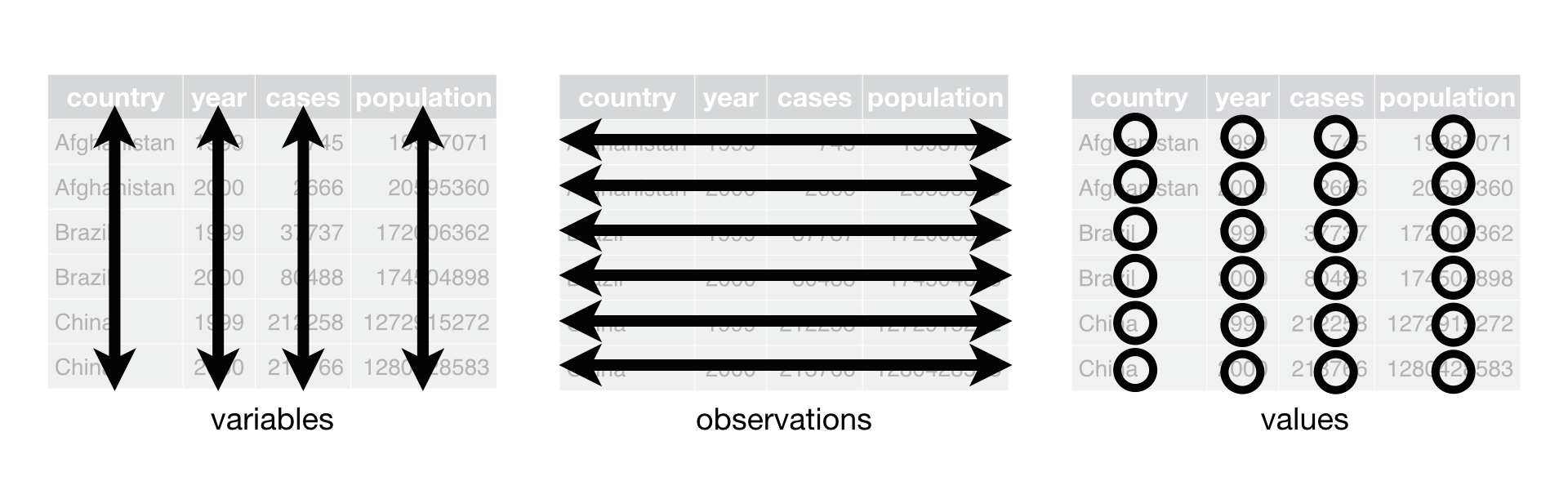
• Each variable is a column
• Each observation is a row
• Each cell is a single value

Is this tidy?

The Billboard dataset: the date a song first entered the Billboard Top 100

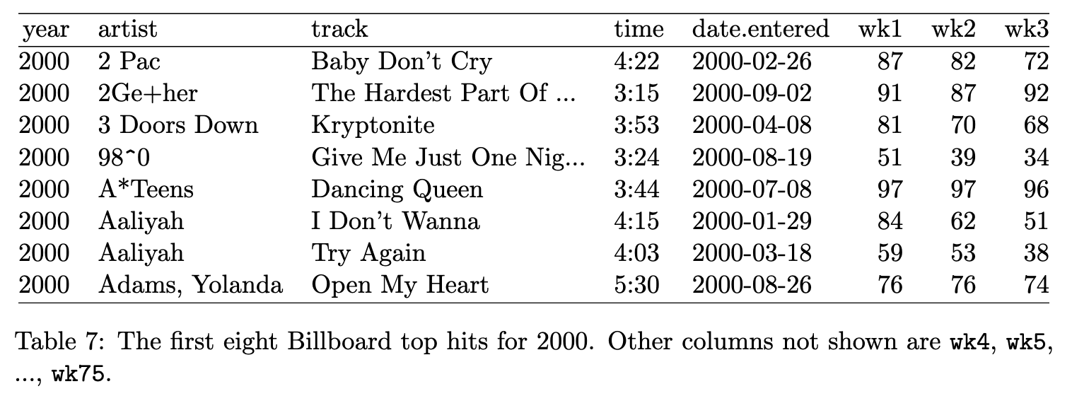
❌: No, because wk1, wk2, … are values, not variables - they should be recorded in cells rather than in column names

Is this tidy?

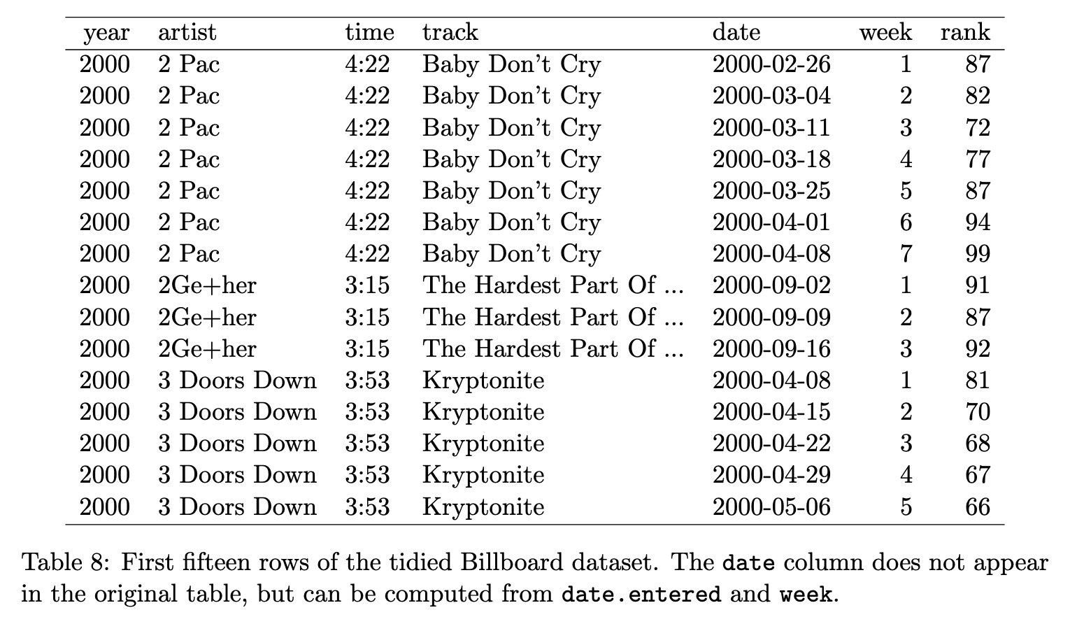
✅ Yes, because 1) The variables are: year, artist, time, track, date, week, and rank, 2) The observation is a recorded rank of a song in a particular week

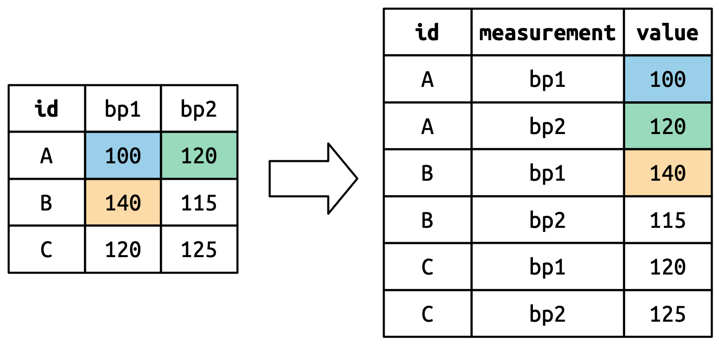
Pivot longer

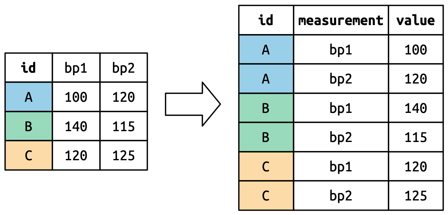
Pivot longer

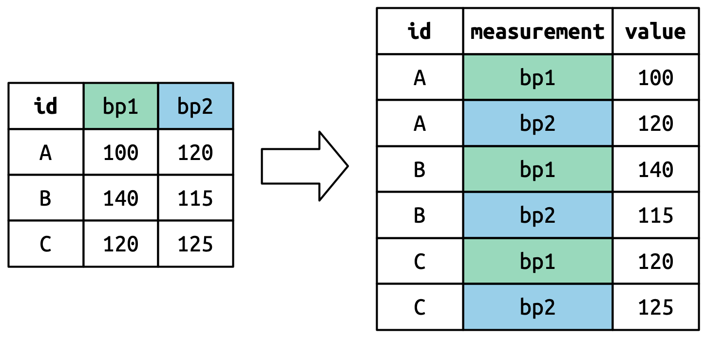
Pivot longer

Pivot longer

Basic syntax:

pivot_longer(cols = columns_to_pivot, 
             names_to = new_colname_to_store_old_column_names, 
             values_to = new_colname_to_store_values))

Example:

df <- tibble(
  id = c("A", "B", "C"),
  bp1 = c(100, 140, 120),
  bp2 = c(120, 115, 125)
)

df

# A tibble: 3 × 3
  id      bp1   bp2
  <chr> <dbl> <dbl>
1 A       100   120
2 B       140   115
3 C       120   125

df |> 
  pivot_longer(
    cols = bp1:bp2,
    names_to = "measurement",
    values_to = "value"
  )

# A tibble: 6 × 3
  id    measurement value
  <chr> <chr>       <dbl>
1 A     bp1           100
2 A     bp2           120
3 B     bp1           140
4 B     bp2           115
5 C     bp1           120
6 C     bp2           125

Your time

usethis::create_from_github("SDS322E-2025FALL/0601-pivot", fork = FALSE)

You can use the full billboard dataset from the tidyr package, but we make it easier by consider only 4 columns and 5 rows.

df <- billboard |> 
  select(artist, track,  wk1, wk2) |> 
  head(5)

df

# A tibble: 5 × 4
  artist       track                     wk1   wk2
  <chr>        <chr>                   <dbl> <dbl>
1 2 Pac        Baby Don't Cry (Keep...    87    82
2 2Ge+her      The Hardest Part Of ...    91    87
3 3 Doors Down Kryptonite                 81    70
4 3 Doors Down Loser                      76    76
5 504 Boyz     Wobble Wobble              57    34

Fill in the blanks to pivot df longer:

df |> 
  pivot_longer(
    cols = ..., 
    names_to = ..., 
    values_to = ...
  )

Your result should look like this:

# A tibble: 10 × 4
   artist       track                   week   rank
   <chr>        <chr>                   <chr> <dbl>
 1 2 Pac        Baby Don't Cry (Keep... wk1      87
 2 2 Pac        Baby Don't Cry (Keep... wk2      82
 3 2Ge+her      The Hardest Part Of ... wk1      91
 4 2Ge+her      The Hardest Part Of ... wk2      87
 5 3 Doors Down Kryptonite              wk1      81
 6 3 Doors Down Kryptonite              wk2      70
 7 3 Doors Down Loser                   wk1      76
 8 3 Doors Down Loser                   wk2      76
 9 504 Boyz     Wobble Wobble           wk1      57
10 504 Boyz     Wobble Wobble           wk2      34

Example - billboard

billboard |> 
  select(artist, track,  wk1, wk2) |> 
  head(5) |> 
  pivot_longer(cols = c(wk1, wk2), names_to = "week", values_to = "rank")

# A tibble: 10 × 4
   artist       track                   week   rank
   <chr>        <chr>                   <chr> <dbl>
 1 2 Pac        Baby Don't Cry (Keep... wk1      87
 2 2 Pac        Baby Don't Cry (Keep... wk2      82
 3 2Ge+her      The Hardest Part Of ... wk1      91
 4 2Ge+her      The Hardest Part Of ... wk2      87
 5 3 Doors Down Kryptonite              wk1      81
 6 3 Doors Down Kryptonite              wk2      70
 7 3 Doors Down Loser                   wk1      76
 8 3 Doors Down Loser                   wk2      76
 9 504 Boyz     Wobble Wobble           wk1      57
10 504 Boyz     Wobble Wobble           wk2      34

You can do exactly the same with all the rows (remove head(5)).

What would you do if you want to pivot all the week columns (wk1, wk2, …, wk76) longer?

Example - billboard

In the full billboard dataset there are 76 weeks: wk1: wk76, we can use starts_with("wk") to select all the columns that start with “wk” (select syntax - week 3 Monday).

billboard |> 
  pivot_longer(
    cols = starts_with("wk"), 
    names_to = "week", 
    values_to = "rank"
  ) 

# A tibble: 24,092 × 5
   artist track                   date.entered week   rank
   <chr>  <chr>                   <date>       <chr> <dbl>
 1 2 Pac  Baby Don't Cry (Keep... 2000-02-26   wk1      87
 2 2 Pac  Baby Don't Cry (Keep... 2000-02-26   wk2      82
 3 2 Pac  Baby Don't Cry (Keep... 2000-02-26   wk3      72
 4 2 Pac  Baby Don't Cry (Keep... 2000-02-26   wk4      77
 5 2 Pac  Baby Don't Cry (Keep... 2000-02-26   wk5      87
 6 2 Pac  Baby Don't Cry (Keep... 2000-02-26   wk6      94
 7 2 Pac  Baby Don't Cry (Keep... 2000-02-26   wk7      99
 8 2 Pac  Baby Don't Cry (Keep... 2000-02-26   wk8      NA
 9 2 Pac  Baby Don't Cry (Keep... 2000-02-26   wk9      NA
10 2 Pac  Baby Don't Cry (Keep... 2000-02-26   wk10     NA
# ℹ 24,082 more rows

Pivot wider

The inverse of pivot longer

Pivot wider

Basic syntax:

pivot_wider(names_from = old_colnames_whose_values_become_the_new_colnames, 
            values_from = old_colnames_whose_values_fill_in_the_cells)

Example:

df <- tibble(
  id = c("A", "B", "B", "A", "A"),
  measurement = c("bp1", "bp1", "bp2", "bp2", "bp3"),
  value = c(100, 140, 115, 120, 105)
)

df

# A tibble: 5 × 3
  id    measurement value
  <chr> <chr>       <dbl>
1 A     bp1           100
2 B     bp1           140
3 B     bp2           115
4 A     bp2           120
5 A     bp3           105

df |> 
  pivot_wider(
    names_from = measurement,
    values_from = value
  )

# A tibble: 2 × 4
  id      bp1   bp2   bp3
  <chr> <dbl> <dbl> <dbl>
1 A       100   120   105
2 B       140   115    NA

Your time

Practice pivot_wider() to get back the original df:

df <- billboard |> 
  select(artist, track,  wk1, wk2) |> 
  head(5) |> 
  pivot_longer(
    cols = c(wk1, wk2), 
    names_to = "week", 
    values_to = "rank"
  )
df

# A tibble: 10 × 4
   artist       track                   week   rank
   <chr>        <chr>                   <chr> <dbl>
 1 2 Pac        Baby Don't Cry (Keep... wk1      87
 2 2 Pac        Baby Don't Cry (Keep... wk2      82
 3 2Ge+her      The Hardest Part Of ... wk1      91
 4 2Ge+her      The Hardest Part Of ... wk2      87
 5 3 Doors Down Kryptonite              wk1      81
 6 3 Doors Down Kryptonite              wk2      70
 7 3 Doors Down Loser                   wk1      76
 8 3 Doors Down Loser                   wk2      76
 9 504 Boyz     Wobble Wobble           wk1      57
10 504 Boyz     Wobble Wobble           wk2      34

Your result should look like this:

# A tibble: 5 × 4
  artist       track                     wk1   wk2
  <chr>        <chr>                   <dbl> <dbl>
1 2 Pac        Baby Don't Cry (Keep...    87    82
2 2Ge+her      The Hardest Part Of ...    91    87
3 3 Doors Down Kryptonite                 81    70
4 3 Doors Down Loser                      76    76
5 504 Boyz     Wobble Wobble              57    34

Your time - solution

billboard |> 
  select(artist, track,  wk1, wk2) |> 
  head(5) |> 
  pivot_longer(cols = c(wk1, wk2), names_to = "week", values_to = "rank") |> 
  pivot_wider(names_from = week, values_from = rank)

# A tibble: 5 × 4
  artist       track                     wk1   wk2
  <chr>        <chr>                   <dbl> <dbl>
1 2 Pac        Baby Don't Cry (Keep...    87    82
2 2Ge+her      The Hardest Part Of ...    91    87
3 3 Doors Down Kryptonite                 81    70
4 3 Doors Down Loser                      76    76
5 504 Boyz     Wobble Wobble              57    34

Recall from visualization lecture 1 …

Anscombe’s quartet

anscombe

   x1 x2 x3 x4    y1   y2    y3    y4
1  10 10 10  8  8.04 9.14  7.46  6.58
2   8  8  8  8  6.95 8.14  6.77  5.76
3  13 13 13  8  7.58 8.74 12.74  7.71
4   9  9  9  8  8.81 8.77  7.11  8.84
5  11 11 11  8  8.33 9.26  7.81  8.47
6  14 14 14  8  9.96 8.10  8.84  7.04
7   6  6  6  8  7.24 6.13  6.08  5.25
8   4  4  4 19  4.26 3.10  5.39 12.50
9  12 12 12  8 10.84 9.13  8.15  5.56
10  7  7  7  8  4.82 7.26  6.42  7.91
11  5  5  5  8  5.68 4.74  5.73  6.89

Summary of average for x and y:

# A tibble: 4 × 3
  set   mean_y mean_x
  <chr>  <dbl>  <dbl>
1 1       7.50      9
2 2       7.50      9
3 3       7.5       9
4 4       7.50      9

Combine pivot_longer and pivot_wider

If we can structure the data into this format…

# A tibble: 44 × 3
   set       x     y
   <chr> <dbl> <dbl>
 1 1        10  8.04
 2 2        10  9.14
 3 3        10  7.46
 4 4         8  6.58
 5 1         8  6.95
 6 2         8  8.14
 7 3         8  6.77
 8 4         8  5.76
 9 1        13  7.58
10 2        13  8.74
# ℹ 34 more rows

then it is easy to map them into x and y axes and facet by set.

dt |> 
  ggplot(aes(x = x, y = y)) + 
  geom_point() + 
  facet_wrap(vars(set))

Combine pivot_longer and pivot_wider

Should we use pivot_wider() or pivot_longer() first?

pivot_longer()!

Start from a tibble:

dt <- rownames_to_column(anscombe, var = "id") |> 
  as_tibble()
dt

# A tibble: 11 × 9
   id       x1    x2    x3    x4    y1    y2    y3    y4
   <chr> <dbl> <dbl> <dbl> <dbl> <dbl> <dbl> <dbl> <dbl>
 1 1        10    10    10     8  8.04  9.14  7.46  6.58
 2 2         8     8     8     8  6.95  8.14  6.77  5.76
 3 3        13    13    13     8  7.58  8.74 12.7   7.71
 4 4         9     9     9     8  8.81  8.77  7.11  8.84
 5 5        11    11    11     8  8.33  9.26  7.81  8.47
 6 6        14    14    14     8  9.96  8.1   8.84  7.04
 7 7         6     6     6     8  7.24  6.13  6.08  5.25
 8 8         4     4     4    19  4.26  3.1   5.39 12.5 
 9 9        12    12    12     8 10.8   9.13  8.15  5.56
10 10        7     7     7     8  4.82  7.26  6.42  7.91
11 11        5     5     5     8  5.68  4.74  5.73  6.89

dt |> 
  pivot_longer(cols = x1: y4, 
               names_to = "variable", 
               values_to = "value") 

# A tibble: 88 × 3
   id    variable value
   <chr> <chr>    <dbl>
 1 1     x1       10   
 2 1     x2       10   
 3 1     x3       10   
 4 1     x4        8   
 5 1     y1        8.04
 6 1     y2        9.14
 7 1     y3        7.46
 8 1     y4        6.58
 9 2     x1        8   
10 2     x2        8   
# ℹ 78 more rows

Combine pivot_longer and pivot_wider

Use separate() to split variable into two columns: type (x or y) and set (1, 2, 3, 4).

• sep = 1 means split at the first position

dt |> 
  pivot_longer(cols = x1: y4, names_to = "variable", values_to = "value") |> 
  separate(variable, into = c("type", "set"), sep = 1)

# A tibble: 88 × 4
   id    type  set   value
   <chr> <chr> <chr> <dbl>
 1 1     x     1     10   
 2 1     x     2     10   
 3 1     x     3     10   
 4 1     x     4      8   
 5 1     y     1      8.04
 6 1     y     2      9.14
 7 1     y     3      7.46
 8 1     y     4      6.58
 9 2     x     1      8   
10 2     x     2      8   
# ℹ 78 more rows

Should we use pivot_wider() or pivot_longer() now?

Combine pivot_longer and pivot_wider

pivot_wider()!

dt |> 
  pivot_longer(cols = x1: y4, names_to = "variable", values_to = "value") |> 
  separate(variable, into = c("type", "set"), sep = 1) |> 
  pivot_wider(names_from = type, values_from = value)

# A tibble: 44 × 4
   id    set       x     y
   <chr> <chr> <dbl> <dbl>
 1 1     1        10  8.04
 2 1     2        10  9.14
 3 1     3        10  7.46
 4 1     4         8  6.58
 5 2     1         8  6.95
 6 2     2         8  8.14
 7 2     3         8  6.77
 8 2     4         8  5.76
 9 3     1        13  7.58
10 3     2        13  8.74
# ℹ 34 more rows

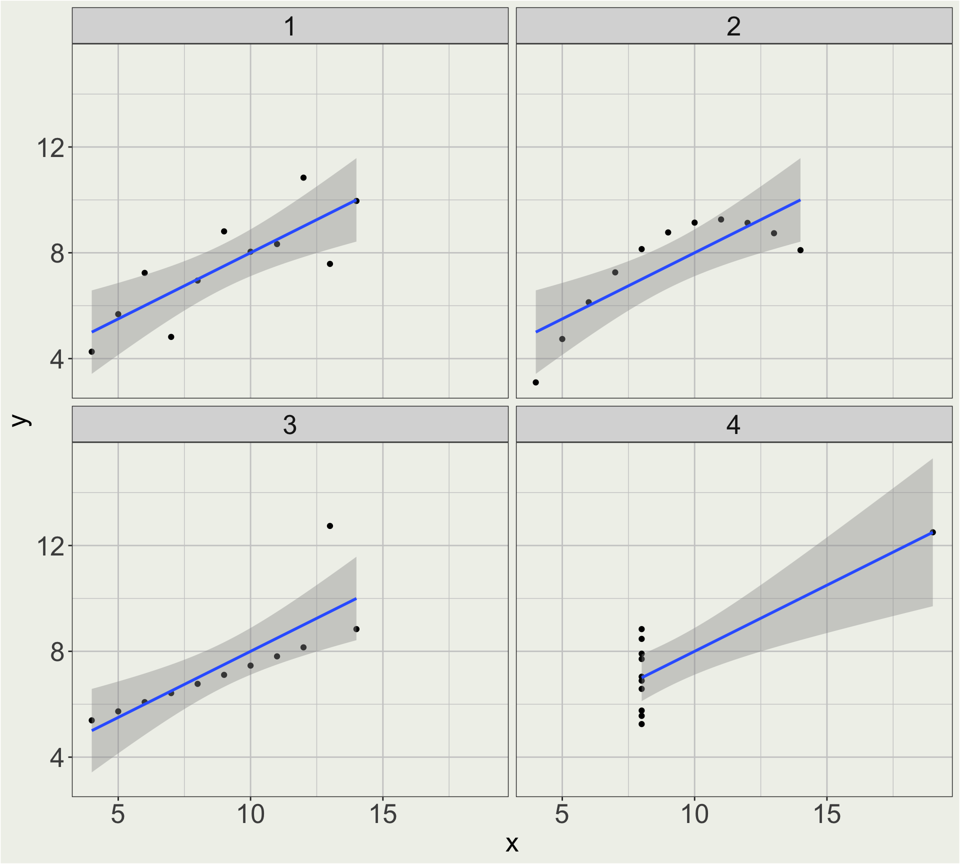
Combine pivot_longer and pivot_wider

Now plot the data!

dt2 <- dt |> 
  pivot_longer(cols = x1: y4, names_to = "variable", values_to = "value") |> 
  separate(variable, into = c("type", "set"), sep = 1) |> 
  pivot_wider(names_from = type, values_from = value)

dt2 |> 
  ggplot(aes(x = x, y = y)) + 
  geom_point() + 
  geom_smooth(method = "lm") + 
  facet_wrap(vars(set), ncol = 2)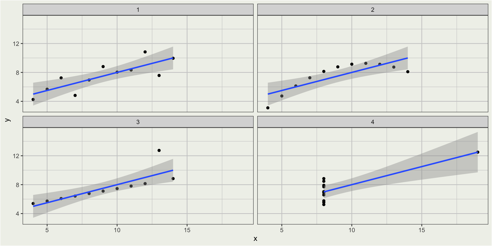 

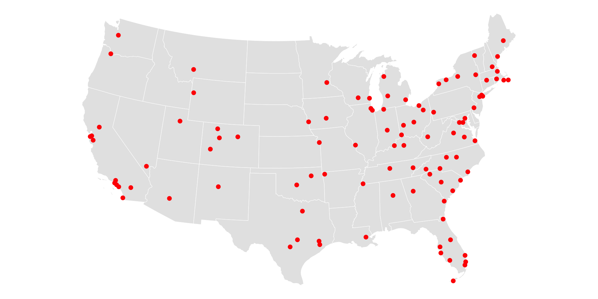
Bonus: plot flight origin and destination on the map

Let’s plot all the origin and destination airports of all the flights in nycflights13::flights on the US map.