Elements of Data Science
SDS 322E

H. Sherry Zhang
Department of Statistics and Data Sciences
The University of Texas at Austin

Fall 2025

Learning objectives

Create date and datetime objects from
- date/ datetime components: make_date(), make_datetime()
- character strings:
  - as_date(), as_datetime() (base version: as.Date())
  - ymd(), mdy(), dmy(), etc
Extract components from date/datetime objects: year(), month(), day(), wday(), yday(), week(), etc
Plot time series data with ggplot2, format axes with date/datetime scales: scale_x_date(), scale_x_datetime()

All sorts of date-time data

flights |>
  select(year, month, day, hour, minute, arr_time, time_hour)

# A tibble: 336,776 × 7
   year month   day  hour minute arr_time time_hour          
  <int> <int> <int> <dbl>  <dbl>    <int> <dttm>             
1  2013     1     1     5     15      830 2013-01-01 05:00:00
2  2013     1     1     5     29      850 2013-01-01 05:00:00
3  2013     1     1     5     40      923 2013-01-01 05:00:00
4  2013     1     1     5     45     1004 2013-01-01 05:00:00
5  2013     1     1     6      0      812 2013-01-01 06:00:00
# ℹ 336,771 more rows

Conversion among:

arguably recognizable datetime characters: “830” for 8:30am
Proper datetime/ date objects: objects of class Date and POSIXct
Components of date times: year, month, day, etc

Create date/datetime objects from components

make_date() combines date components into a Date object.

flights |>
  mutate(depature = make_date(year, month, day), .keep = "used")

# A tibble: 336,776 × 4
   year month   day depature  
  <int> <int> <int> <date>    
1  2013     1     1 2013-01-01
2  2013     1     1 2013-01-01
3  2013     1     1 2013-01-01
4  2013     1     1 2013-01-01
5  2013     1     1 2013-01-01
# ℹ 336,771 more rows

make_datetime() creates a date-time object from individual components.

flights |>
  mutate(depature = make_datetime(year, month, day, hour, minute), .keep = "used")

# A tibble: 336,776 × 6
   year month   day  hour minute depature           
  <int> <int> <int> <dbl>  <dbl> <dttm>             
1  2013     1     1     5     15 2013-01-01 05:15:00
2  2013     1     1     5     29 2013-01-01 05:29:00
3  2013     1     1     5     40 2013-01-01 05:40:00
4  2013     1     1     5     45 2013-01-01 05:45:00
5  2013     1     1     6      0 2013-01-01 06:00:00
# ℹ 336,771 more rows

Example: construct depature time

flights |>
  mutate(
    hour = dep_time %/% 100,
    minute = dep_time %% 100,
    dep_time2 = make_datetime(year = year, month = month, day = day, hour = hour, min = minute),
    .keep = "used")

# A tibble: 336,776 × 7
   year month   day dep_time  hour minute dep_time2          
  <int> <int> <int>    <int> <dbl>  <dbl> <dttm>             
1  2013     1     1      517     5     17 2013-01-01 05:17:00
2  2013     1     1      533     5     33 2013-01-01 05:33:00
3  2013     1     1      542     5     42 2013-01-01 05:42:00
4  2013     1     1      544     5     44 2013-01-01 05:44:00
5  2013     1     1      554     5     54 2013-01-01 05:54:00
# ℹ 336,771 more rows

%/% is integer division, %% is modulo operation (remainder after division). They are base R arithmetic operators.

Create date objects from character strings

as.Date() (base) or as_date() (lubridate) converts character strings to Date objects.

"2020-01-01"

[1] "2020-01-01"

as.Date("2020-01-01")

[1] "2020-01-01"

Although the prints are identical before and after, they are internally treated differently (they have different classes). We can check with class():

class(as.Date("2020-01-01"))

[1] "Date"

class("2020-01-01")

[1] "character"

Create datetime objects from character strings

"2020-01-02 03:04:05"

[1] "2020-01-02 03:04:05"

our_datetime <- as_datetime("2020-01-02 03:04:05")
our_datetime

[1] "2020-01-02 03:04:05 UTC"

class(our_datetime)

[1] "POSIXct" "POSIXt"

Here POSIXct is a date-time class that represents the number of seconds since 1970-01-01 (the “epoch”). Sometimes you may also see POSIXlt in the wild, which is a list-based date-time class (stores a list of date-time components).

This is also how the time_hour variable stored in nycflights13::flights dataset:

flights |> select(time_hour) |> head(1)

# A tibble: 1 × 1
  time_hour          
  <dttm>             
1 2013-01-01 05:00:00

class(flights$time_hour)

[1] "POSIXct" "POSIXt"

Convert from a proper time object to time components

These are vector functions from the lubridate package

our_datetime

[1] "2020-01-02 03:04:05 UTC"

year(our_datetime)

[1] 2020

month(our_datetime)

[1] 1

month(our_datetime, label = TRUE)

[1] Jan
12 Levels: Jan < Feb < Mar < Apr < May < Jun < Jul < Aug < Sep < ... < Dec

day(our_datetime)

[1] 2

hour(our_datetime)

[1] 3

minute(our_datetime)

[1] 4

second(our_datetime)

[1] 5

wday(our_datetime)

[1] 5

yday(our_datetime)

[1] 2

week(our_datetime)

[1] 1

Example: extract time components out of a datetime object

They can be used inside mutate() to extract components from a date-time variable:

flights |> 
  mutate(
    year = year(time_hour),
    month = month(time_hour, label = TRUE),
    day = day(time_hour),
    hour = hour(time_hour),
    minute = minute(time_hour),
    wday = wday(time_hour, label = TRUE),
    yday = yday(time_hour),
    week = week(time_hour),
    .keep = "used"
  )

# A tibble: 336,776 × 9
   year month   day  hour minute time_hour           wday   yday  week
  <dbl> <ord> <int> <int>  <int> <dttm>              <ord> <dbl> <dbl>
1  2013 Jan       1     5      0 2013-01-01 05:00:00 Tue       1     1
2  2013 Jan       1     5      0 2013-01-01 05:00:00 Tue       1     1
3  2013 Jan       1     5      0 2013-01-01 05:00:00 Tue       1     1
4  2013 Jan       1     5      0 2013-01-01 05:00:00 Tue       1     1
5  2013 Jan       1     6      0 2013-01-01 06:00:00 Tue       1     1
# ℹ 336,771 more rows

Parse date-time from character strings

If your date/ datetime character strings are in relatively standard format, there are shortcuts:

ymd("2020-01-01")

[1] "2020-01-01"

class(ymd("2020-01-01"))

[1] "Date"

mdy("01-31-2020")

[1] "2020-01-31"

dmy("31-01-2020")

[1] "2020-01-31"

ymd_h("2020-01-01 05")

[1] "2020-01-01 05:00:00 UTC"

ymd_hm("2020-01-01 05:01")

[1] "2020-01-01 05:01:00 UTC"

ymd_hms("2020-01-01 05:01:02")

[1] "2020-01-01 05:01:02 UTC"

Example: ggplot2 downloads over time

pkg_df <- cranlogs::cran_downloads(
  packages = "ggplot2",
  from = "2024-01-01", to = "2024-12-31") |>
  as_tibble()
pkg_df

# A tibble: 366 × 3
  date       count package
  <date>     <dbl> <chr>  
1 2024-01-01 51694 ggplot2
2 2024-01-02 67030 ggplot2
3 2024-01-03 71770 ggplot2
4 2024-01-04 71122 ggplot2
5 2024-01-05 66201 ggplot2
# ℹ 361 more rows

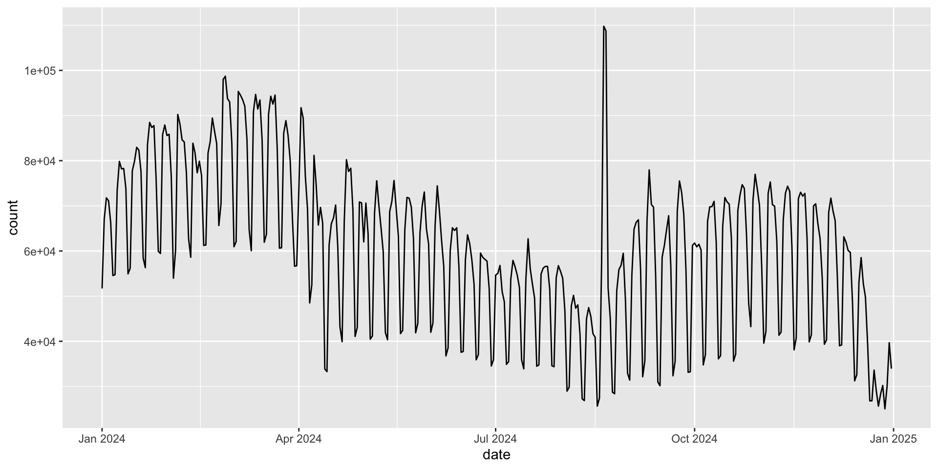
Example: ggplot2 downloads over time

pkg_df |>
  ggplot(aes(x = date, y = count)) +
  geom_line()

Maybe the y-axis can be formatted better 🤔 - where do you think we should go to change the y-axis labels?

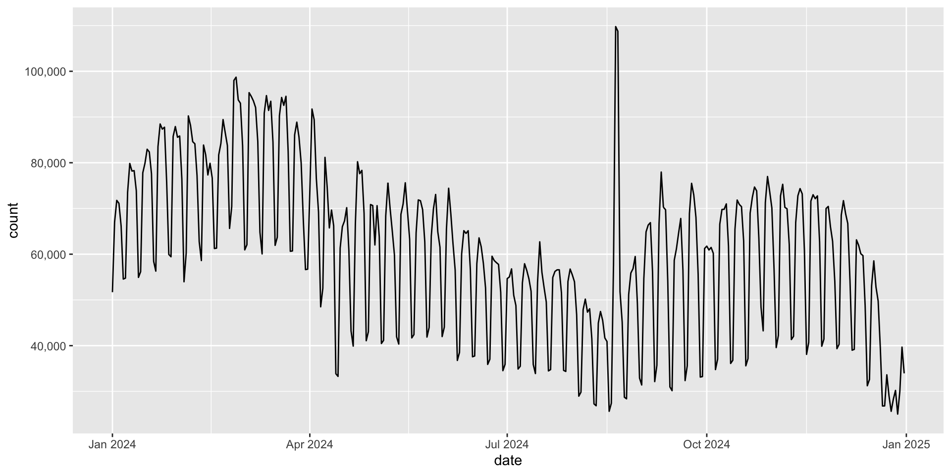
Example: ggplot2 downloads over time

Similar to the labeling in facets, we can use scale_y_continuous(labels = ...) to format the y-axis labels.

pkg_df |>
  ggplot(aes(x = date, y = count)) +
  geom_line() + 
  scale_y_continuous(labels = scales::label_comma())

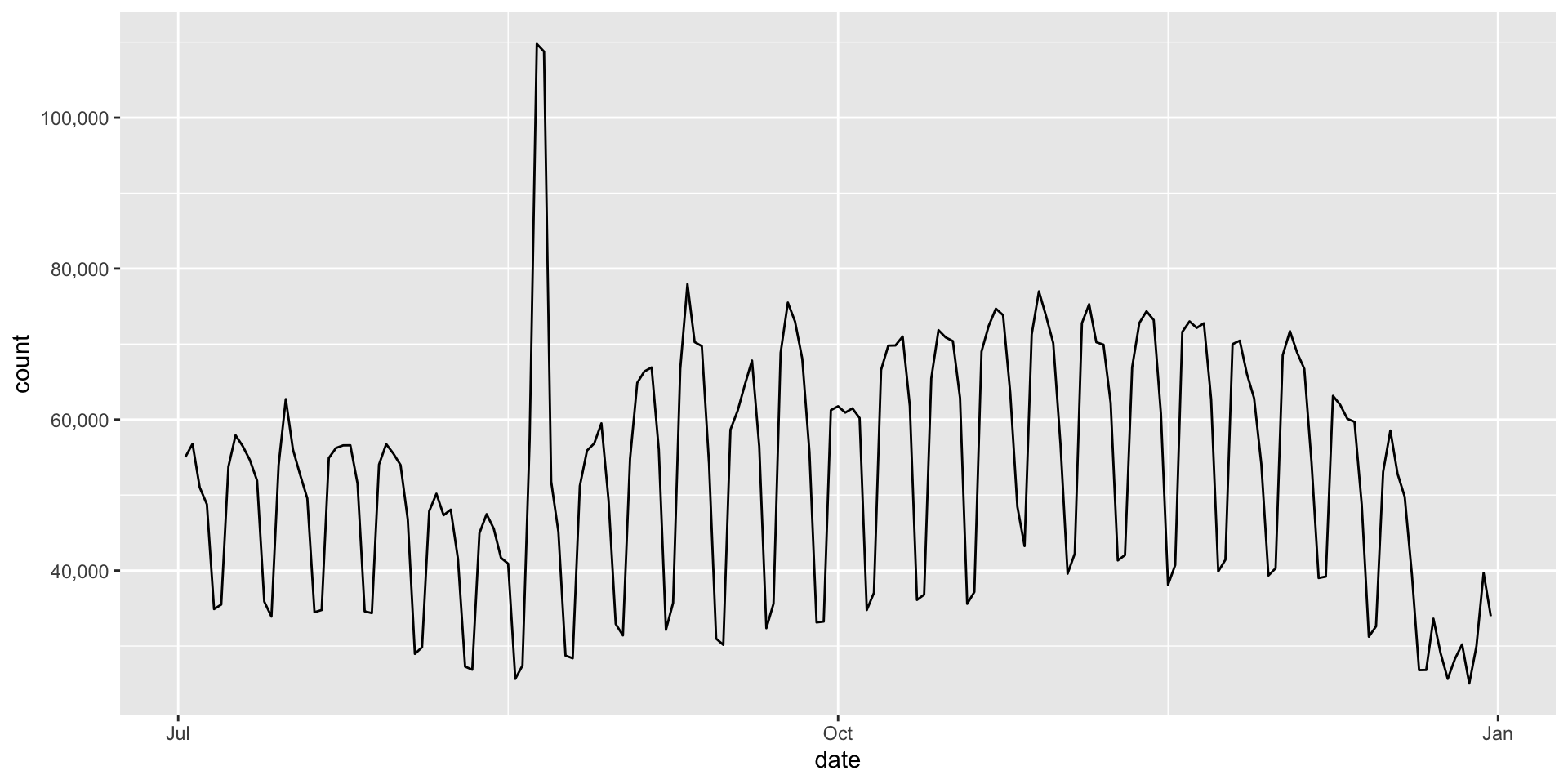
Zoom in for the second half of the year

pkg_df |>
  filter(date > as.Date("2024-07-01")) |>
  ggplot(aes(x = date, y = count)) +
  geom_line() + 
  scale_y_continuous(labels = scales::label_comma())

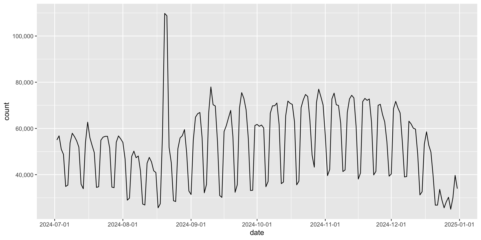
Maybe we want to format the x-axis better 🤔

scale_x_date

You can change the number of breaks in scale_x_date() with literal text:

date_breaks = "1 month" (or "2 weeks", "3 days", etc)

pkg_df |>
  filter(date > as.Date("2024-07-01")) |>
  ggplot(aes(x = date, y = count)) +
  geom_line() +
  scale_y_continuous(labels = scales::label_comma()) + 
  scale_x_date(date_breaks = "1 month")

scale_x_date

You can change the labels in scale_x_date() with date_labels = "..." (see next slide for a list of options)

pkg_df |>
  filter(date > as.Date("2024-07-01")) |>
  ggplot(aes(x = date, y = count)) +
  geom_line() +
  scale_y_continuous(labels = scales::label_comma()) + 
  scale_x_date(date_breaks = "1 month", date_labels = "%Y %b")

A list of date labels

Type	Code	Meaning	Example
Year	`%Y`	4 digit year	2021
	`%y`	2 digit year	21
Month	`%m`	Number	2
	`%b`	Abbreviated name	Feb
	`%B`	Full name	February
Day	`%d`	One or two digits	2
	`%e`	Two digits	02
Time	`%H`	24-hour hour	13
	`%I`	12-hour hour	1
	`%M`	Minutes	35
	`%S`	Seconds	45

One more example

You can also add other symbols, such as -, / in the date_labels argument.

pkg_df |>
  filter(date > as.Date("2024-07-01")) |>
  ggplot(aes(x = date, y = count)) +
  geom_line() +
  scale_y_continuous(labels = scales::label_comma()) + 
  scale_x_date(date_breaks = "1 month", date_labels = "%y-%b")

Your time

usethis::create_from_github("SDS322E-2025FALL/0502-datetime", fork = FALSE)

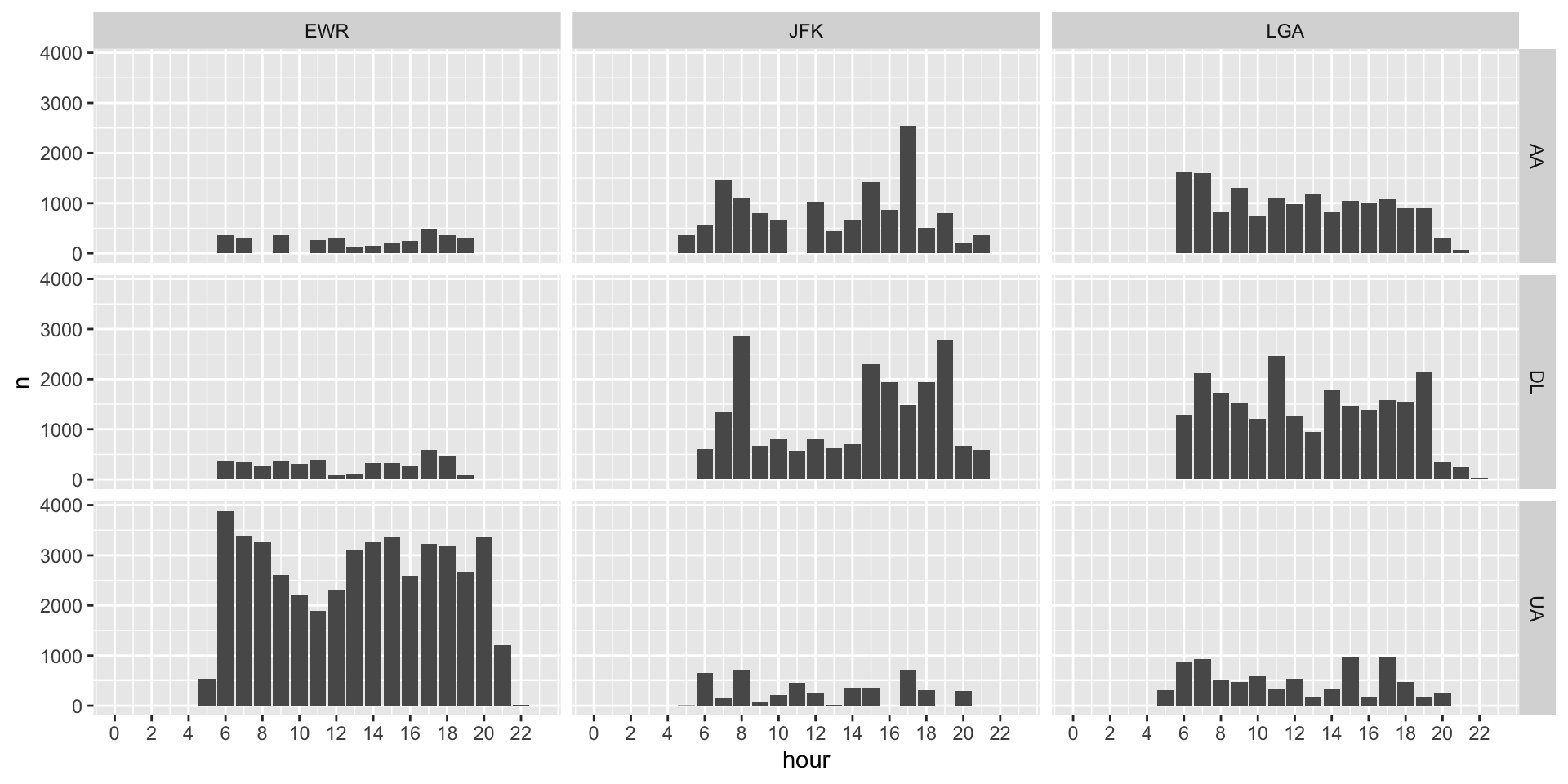
Let’s look at the flights data again, focus only on three carrier: AA, DL, and UA. We can make a plot of the hourly count of flights for each carrier at each of the three airports in NY (EWR, JFK, LGA).

You may start from the following code:

df <- flights |>
  # step 1: focus on three carriers
  ...
  # step 2: count number of flights by carrier, origin, and hour
  ...

df |>
  ggplot(aes(...)) +
  geom_col() +
  # when you want to facet by two variables
  facet_grid(...) +
  # similar to scale_x_date(), with regular scale_x_continuous, you can change the breaks and limits
  # here I ask for a break every 2 hours, and limit the x-axis to be between 0 and 23 
  # (so we can see there are no midnight flights)
  scale_x_continuous(breaks = seq(0, 23, by = 2), limits = c(0, 23))

Solution

df <- flights |>
  filter(carrier %in% c("AA", "DL", "UA")) |>
  count(carrier, origin, hour)

df |>
  ggplot(aes(x = hour, y = n)) +
  geom_col() +
  facet_grid(carrier ~ origin) +
  scale_x_continuous(breaks = seq(0, 23, by = 2), limits = c(0, 23))

Of course, you can keep building on this to make the facet header more informative, change the y-axis labels, etc.

Elements of Data Science SDS 322E

Learning objectives

All sorts of date-time data

Create date/datetime objects from components

Example: construct depature time

Create date objects from character strings

Create datetime objects from character strings

Convert from a proper time object to time components

Example: extract time components out of a datetime object

Parse date-time from character strings

Example: ggplot2 downloads over time

Example: ggplot2 downloads over time

Example: ggplot2 downloads over time

Zoom in for the second half of the year

scale_x_date

scale_x_date

A list of date labels

One more example

Your time

Solution

Elements of Data Science
SDS 322E