Elements of Data Science
SDS 322E

H. Sherry Zhang
Department of Statistics and Data Sciences
The University of Texas at Austin

Fall 2025

Learning objective

Apart from the mutate(), filter(), group_by(), summarize(), and arrange(), we introduced last week, there are a few others you should know about:

select(): Keep or drop columns using their names and types (select by column)
slice(): Subset rows using their positions (select by rows)
rename(): rename variables
functions that can be used to construct more complicated expression and predicate functions inside mutate() and filter():
- between(): a convenient way to filter by a range
- if_else()/ ifelse(): create a new variable based on a condition
- case_when(): create a new variable based on multiple conditions

And more…

`select()`: Keep or drop columns using their names and types

`select()` syntax

DATA |> select(...)

Select takes a data frame as an input, keep the column selected, and output a data frame

flights |> select(dep_delay)

# A tibble: 336,776 × 1
   dep_delay
       <dbl>
 1         2
 2         4
 3         2
 4        -1
 5        -6
 6        -4
 7        -5
 8        -3
 9        -3
10        -2
# ℹ 336,766 more rows

`select()` syntax

DATA |> select(...)

# select by variable name(s)
flights |> select(year)
flights |> select(year:dep_delay)

# select by position
flights |> select(1:4)
flights |> select(c(1, 3:5))

# remove certain variables
flights |> select(-year, -month, -day)
flights |> select(c(1, 3:5), -4) # select 1, 3, 5

# select by selectors
flights |> select(starts_with(c("dep", "arr"))) 
flights |> select(ends_with("time")) 
flights |> select(contains(c("dep", "arr")))

`select()`: a little more about the selectors:

colnames(flights)

 [1] "year"           "month"          "day"            "dep_time"      
 [5] "sched_dep_time" "dep_delay"      "arr_time"       "sched_arr_time"
 [9] "arr_delay"      "carrier"        "flight"         "tailnum"       
[13] "origin"         "dest"           "air_time"       "distance"      
[17] "hour"           "minute"         "time_hour"

flights |> select(starts_with(c("dep", "arr")))

dep_time, dep_delay, arr_time, arr_delay

flights |> select(ends_with("time"))

dep_time, sched_dep_time, arr_time, sched_arr_time, air_time

flights |> select(contains(c("dep", "arr")))

dep_time, sched_dep_time, dep_delay, arr_time, sched_arr_time, arr_delay, carrier

`slice()`: Subset rows using their positions

`slice()` syntax

flights |> slice(1:10)

# slice the first/ last few rows
flights |> slice_head(n = 10) # same as slice()
flights |> slice_tail(n = 5) 

# slice the rows with largest/ smallest n values of a variable
flights |> slice_max(dep_delay) # what's the by default value?
flights |> slice_max(dep_delay, n = 10)
flights |> slice_min(distance, n = 5)

# slice through a random sample
flights |> slice_sample(n = 10)

`slice_sample()`: when randomness comes in

v1 <- flights |> slice_sample(n = 10)
v2 <- flights |> slice_sample(n = 10)

v1

# A tibble: 10 × 19
    year month   day dep_time sched_dep_time
   <int> <int> <int>    <int>          <int>
 1  2013     3    26      846            615
 2  2013     8    26     1929           1940
 3  2013     2    19     1113           1114
 4  2013     8     3     1515           1455
 5  2013     3    15     1759           1800
 6  2013     6     2     2213           1816
 7  2013     3     5     1413           1420
 8  2013     7     4     1355           1355
 9  2013     5    19      556            600
10  2013     4    14      701            705
# ℹ 14 more variables: dep_delay <dbl>,
#   arr_time <int>, sched_arr_time <int>,
#   arr_delay <dbl>, carrier <chr>, flight <int>,
#   tailnum <chr>, origin <chr>, dest <chr>,
#   air_time <dbl>, distance <dbl>, hour <dbl>,
#   minute <dbl>, time_hour <dttm>

v2

# A tibble: 10 × 19
    year month   day dep_time sched_dep_time
   <int> <int> <int>    <int>          <int>
 1  2013    12    14     1358           1355
 2  2013     3    25     1613           1600
 3  2013     7    12     1414           1417
 4  2013     9     5     1624           1615
 5  2013     7    22      757            800
 6  2013     4    14     1223           1200
 7  2013    11    25     1153           1155
 8  2013    12    28      803            735
 9  2013     5    10      826            830
10  2013     3    14      555            600
# ℹ 14 more variables: dep_delay <dbl>,
#   arr_time <int>, sched_arr_time <int>,
#   arr_delay <dbl>, carrier <chr>, flight <int>,
#   tailnum <chr>, origin <chr>, dest <chr>,
#   air_time <dbl>, distance <dbl>, hour <dbl>,
#   minute <dbl>, time_hour <dttm>

identical(v1, v2)

[1] FALSE

`slice_sample()`: when randomness comes in

slice_sample() is your first random function in this course. Random means when you run it multiple times, you get different answers, even all the inputs are the same.

This is not surprising because some functions are designed to be random, e.g. generate random variables (rnorm() - generate normal random variables - there are functions for generate most commonly used distributions).

But it is not useful if we get different results every time because they won’t be reproducible.
Ideally we want these functions to be random, but if we rerun it multiple times, we want to get the same answer.

This is what set.seed() does - it “fixes the randomness”

`set.seed()` Syntax

set.seed(seed = NUMBER)

set.seed(123), set.seed(1), set.seed(20250908), etc all work
The results will be the same for the same seed, but different for different seeds.

There is no output when you run the set.seed() function.

set.seed(123)

But the next command after set.seed() will be deterministic with the same seed.

set.seed(123)
v1 <- flights |> slice_sample(n = 10)

set.seed(123)
v2 <- flights |> slice_sample(n = 10)
identical(v1, v2)

[1] TRUE

`set.seed()`: Common mistake #1

You need to run set.seed() before every random function to guarantee it’s reproducibility:

# now let's "fix the randomness" through setting a seed
set.seed(123)
v1 <- flights |> slice_sample(n = 10)

v2 <- flights |> slice_sample(n = 10)
identical(v1, v2)

[1] FALSE

`set.seed()`: Common mistake #2

With different seeds, your result won’t be fixed:

# now let's "fix the randomness" through setting a seed
set.seed(123)
v1 <- flights |> slice_sample(n = 10)

set.seed(1234)
v2 <- flights |> slice_sample(n = 10)
identical(v1, v2)

[1] FALSE

`sample_n()`: another way to get a random sample of rows

DATA |> sample_n(...)

flights |> sample_n(10)

# A tibble: 10 × 19
    year month   day dep_time sched_dep_time
   <int> <int> <int>    <int>          <int>
 1  2013     7    31      853            853
 2  2013     6    17      956           1000
 3  2013     6     8     2358           2359
 4  2013     4    17       NA            720
 5  2013     5    26     1232           1235
 6  2013     3    30     1926           1930
 7  2013     9     3     1453           1459
 8  2013     9    24      802            805
 9  2013     2    24     1425           1400
10  2013    10    21     1748           1755
# ℹ 14 more variables: dep_delay <dbl>,
#   arr_time <int>, sched_arr_time <int>,
#   arr_delay <dbl>, carrier <chr>, flight <int>,
#   tailnum <chr>, origin <chr>, dest <chr>,
#   air_time <dbl>, distance <dbl>, hour <dbl>,
#   minute <dbl>, time_hour <dttm>

`sample_n()`: why this code below doesn’t work?

flights |> sample_n(n = 10)

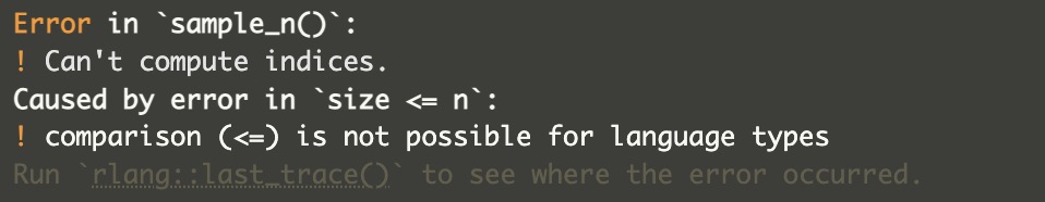
Your time:

Grab the repository:

usethis::create_from_github("SDS322E-2025FALL/0301-dplyr2", fork = FALSE)

Look up the documentation for sample_n and find the proper argument name for the number of sample.

# use ?sample_n to find the correct why to get a random sample of 10 rows
flights |> sample_n(... = 10)

What does the documentation says about the current status of the function sample_n()? What is the current recommendation? Can you see why?

`rename()`: Rename columns

`rename()` syntax

DATA |> rename(NEW_NAME = OLD_NAME, ...)

gapminder::gapminder

# A tibble: 1,704 × 6
   country     continent  year lifeExp      pop
   <fct>       <fct>     <int>   <dbl>    <int>
 1 Afghanistan Asia       1952    28.8  8425333
 2 Afghanistan Asia       1957    30.3  9240934
 3 Afghanistan Asia       1962    32.0 10267083
 4 Afghanistan Asia       1967    34.0 11537966
 5 Afghanistan Asia       1972    36.1 13079460
 6 Afghanistan Asia       1977    38.4 14880372
 7 Afghanistan Asia       1982    39.9 12881816
 8 Afghanistan Asia       1987    40.8 13867957
 9 Afghanistan Asia       1992    41.7 16317921
10 Afghanistan Asia       1997    41.8 22227415
# ℹ 1,694 more rows
# ℹ 1 more variable: gdpPercap <dbl>

gapminder::gapminder |> rename(life_exp = lifeExp)

# A tibble: 1,704 × 6
   country     continent  year life_exp      pop
   <fct>       <fct>     <int>    <dbl>    <int>
 1 Afghanistan Asia       1952     28.8  8425333
 2 Afghanistan Asia       1957     30.3  9240934
 3 Afghanistan Asia       1962     32.0 10267083
 4 Afghanistan Asia       1967     34.0 11537966
 5 Afghanistan Asia       1972     36.1 13079460
 6 Afghanistan Asia       1977     38.4 14880372
 7 Afghanistan Asia       1982     39.9 12881816
 8 Afghanistan Asia       1987     40.8 13867957
 9 Afghanistan Asia       1992     41.7 16317921
10 Afghanistan Asia       1997     41.8 22227415
# ℹ 1,694 more rows
# ℹ 1 more variable: gdpPercap <dbl>

More complicated expressions inside `mutate()` and `filter()`

between()
if_else()/ ifelse()
case_when()

`between()`: a convenient way to filter by a range

syntax: between(VALUE, LEFT, RIGHT)

between(1:5, 2, 3) # for numbers 1:5, output TRUE/ FALSE value to indicate whether each number is between 2 and 3 (inclusive)

[1] FALSE  TRUE  TRUE FALSE FALSE

Because it is a predicate function (output TRUE/ FALSE), we can use it inside filter(), e.g. for the dep_delay variable, output whether each value is between 60 and 120 (inclusive)

v1 <- flights |> filter(between(dep_delay, 60, 120))
v1

# A tibble: 17,336 × 19
   year month   day dep_time sched_dep_time dep_delay arr_time sched_arr_time
  <int> <int> <int>    <int>          <int>     <dbl>    <int>          <int>
1  2013     1     1      811            630       101     1047            830
2  2013     1     1      826            715        71     1136           1045
3  2013     1     1     1120            944        96     1331           1213
4  2013     1     1     1301           1150        71     1518           1345
# ℹ 17,332 more rows
# ℹ 11 more variables: arr_delay <dbl>, carrier <chr>, flight <int>,
#   tailnum <chr>, origin <chr>, dest <chr>, air_time <dbl>, distance <dbl>,
#   hour <dbl>, minute <dbl>, time_hour <dttm>

v2 <- flights |> filter(dep_delay >= 60, dep_delay <= 120)
identical(v1, v2)

[1] TRUE

`ifelse()` and its dplyr brother `if_else()`

syntax: ifelse(PREDICATE, VALUE_IF_TRUE, VALUE_IF_FALSE)

ifelse(1:4 <= 2, "smaller than or equal to 2", "larger than 2")

[1] "smaller than or equal to 2" "smaller than or equal to 2"
[3] "larger than 2"              "larger than 2"

We can use ifelse() inside mutate() to create new variables based on existing variables, e.g. if the departure delay is less than or equal to 20 minutes, it is “on time”; otherwise, it is “delayed”

flights |> mutate(
  delay_status = ifelse(dep_delay > 20, "delayed", "on time"),
  .keep = "used"
)

# A tibble: 336,776 × 2
  dep_delay delay_status
      <dbl> <chr>       
1         2 on time     
2         4 on time     
3         2 on time     
4        -1 on time     
# ℹ 336,772 more rows

Think of ifelse() and if_else() as interchangeable.

`case_when()` syntax

case_when(CONDITION1 ~ VALUE1, 
          CONDITION2 ~ VALUE2,
          ..., 
          TRUE ~ DEFAULT_VALUE)

If you just use ifelse(() 😿:

ifelse(CONDITION1, vALUE1, ifelse(CONDITION2, VALUE2, ifelse(..., DEFAULT_VALUE)))

Example:

flights |>
  mutate(delay_status = case_when(
    dep_delay <= 20 ~ "on time",
    between(dep_delay, 21, 60) ~ "<1r delayed",
    between(dep_delay, 61, 120) ~ "2r delayed",
    TRUE ~ "more than 2r delayed"
  ),.keep = "used")

# A tibble: 336,776 × 2
  dep_delay delay_status
      <dbl> <chr>       
1         2 on time     
2         4 on time     
3         2 on time     
4        -1 on time     
# ℹ 336,772 more rows

A few ways to reenforce today’s lesson

The dplyr pkgdown site
- Get Start page: https://dplyr.tidyverse.org/articles/dplyr.html
- article Grouped data: https://dplyr.tidyverse.org/articles/grouping.html
R for Data Science textbook:
- Chapter 3 Data transformation: https://r4ds.hadley.nz/data-transform.html
- Chapter 12 Logical vectors: https://r4ds.hadley.nz/logicals.html
- Chapter 13 Numbers: https://r4ds.hadley.nz/numbers.html
Statistical Computing using R and Python:
- Chapter 22 Data cleaning: https://srvanderplas.github.io/stat-computing-r-python/part-wrangling/03-data-cleaning.html
  - look at the R dplyr tab for code

What do I mean by …?

These are the fundamentals for building up more complex data wrangling… (Week 2 Friday lecture slide 4)

A code snippet from week 8 case study:

flight_df |>
  filter(!is.na(DepTime), !is.na(ArrTime)) |>
  filter((Origin == airport_vec | Dest == airport_vec), Reporting_Airline == "AA") |>
  mutate(DepTime = as_datetime(paste0("2019-01-01", "-", DepTime, "-00")),
         ArrTime = as_datetime(paste0("2019-01-01", "-", ArrTime, "-00"))) |>
  rename(dep_time = DepTime, arr_time = ArrTime, airline = Reporting_Airline,
         dep_airport = Origin, arr_airport = Dest) |>
  pivot_longer(cols = -c(FlightDate, airline), names_to = c("type", ".value"), names_sep = "_") |>
  filter(airport %in% airport_vec) |>
  mutate(block = assign_time_blocks(time, 10)) |>
  count(airline, airport, type, block) |>
  mutate(airline_airport = paste(airline, airport, sep = "/ "), n = ifelse(type == "dep", n, -n))

Technically you’ve learnt how to filter(), mutate(), rename(), count(), ifelse(), ==, |, !, is.na(), c(), %in%, etc.

We will be learning date and time (as_datetime()) in Week 4 and tidying data (pivot_longer()) in Week 5.

Of course, your assessment will be way simple than this :)

Bonus: try this question

With the mtcars data:

Convert the mpg variable into kpl (1 mpg = 0.425144 km/l)
Only look at V-shaped engine Hint: look at the documentation to see what this means
Find the average kpl and disp for each number of cylinders
Arrange the result by disp in descending order

Elements of Data Science SDS 322E

Learning objective

select(): Keep or drop columns using their names and types

select() syntax

select() syntax

select(): a little more about the selectors:

slice(): Subset rows using their positions

slice() syntax

slice_sample(): when randomness comes in

slice_sample(): when randomness comes in

set.seed() Syntax

set.seed(): Common mistake #1

set.seed(): Common mistake #2

sample_n(): another way to get a random sample of rows

sample_n(): why this code below doesn’t work?

Your time:

rename(): Rename columns

rename() syntax

More complicated expressions inside mutate() and filter()

between(): a convenient way to filter by a range

ifelse() and its dplyr brother if_else()

case_when() syntax

A few ways to reenforce today’s lesson

What do I mean by …?

Of course, your assessment will be way simple than this :)

Bonus: try this question

Elements of Data Science
SDS 322E

`select()`: Keep or drop columns using their names and types

`select()` syntax

`select()` syntax

`select()`: a little more about the selectors:

`slice()`: Subset rows using their positions

`slice()` syntax

`slice_sample()`: when randomness comes in

`slice_sample()`: when randomness comes in

`set.seed()` Syntax

`set.seed()`: Common mistake #1

`set.seed()`: Common mistake #2

`sample_n()`: another way to get a random sample of rows

`sample_n()`: why this code below doesn’t work?

`rename()`: Rename columns

`rename()` syntax

More complicated expressions inside `mutate()` and `filter()`

`between()`: a convenient way to filter by a range

`ifelse()` and its dplyr brother `if_else()`

`case_when()` syntax