Elements of Data Science
SDS 322E

H. Sherry Zhang
Department of Statistics and Data Sciences
The University of Texas at Austin

Fall 2025

Upcoming assessment

Item	Available	Due	Mode
Lab 1	Week 3 Mon Sep 8 12am	Week 3 Mon Sep 8 11:59pm	Complete during the lab session in your lab group
HW 1	Week 3 Thur Sep 11 12am	Week 4 Thur Sep 18 11:59pm	Complete individually
Lab 2	Week 4 Mon Sep 15 12am	Week 4 Mon Sep 15 11:59pm	Complete during the lab session in your lab group
HW 2	Week 4 Thur Sep 18 12am	Week 5 Thur Sep 25 11:59pm	Complete individually
Lab 3	Week 5 Mon Sep 22 12am	Week 5 Mon Sep 22 11:59pm	Complete during the lab session in your lab group
HW 3	Week 5 Thur Sep 25 12am	Week 6 Thur Oct 02 11:59pm	Complete individually

See canvas for lab group allocation

Seek helps during the office hours

GDC (Gates Dell Complex) level 7 open space

Monday 10-12pm after class with me
Monday 6-7pm with Daniel Wang (UGCA)
Tuesday 2-3:15pm with Luke Bellinger (UGCA)
Wednesday 3-5pm with Arka Sinha (Grad TA)
Friday 10-11am with Luke Bellinger (UGCA)

Learning objective

We will learn the five most basic dplyr verbs to wrangle data, including:

filter(): filter rows by a predicate
mutate(): create or modify variables
group_by(): group data by one or more variables
summarize(): summarize data by groups
arrange(): sort data by one or more variables

These are the fundamentals for building up more complex data wrangling…

By the end of the class, you are expected to write code to answer question like this:

Task: We want to summarize the proportion of flights with departure delay larger than 2 hours.

`dplyr` syntax

DATA |> filter(PREDICATE) Predicate functions produce a TRUE or FALSE output.

a == b means whether a is equal to b
a != b means whether a is NOT equal to b

1 == 1

[1] TRUE

1 == 2

[1] FALSE

1 != 2

[1] TRUE

`dplyr` syntax

Predicate functions produce a TRUE or FALSE output.

When the right hand side is not a single number, you need %in%

a %in% c(x1, x2, ...) means whether a is one of the values in the vector c(x1, x2, ...)
!a %in% c(x1, x2, ...) means whether a is NOT one of the values in the vector c(x1, x2, ...)

3 %in% c(1, 2)

[1] FALSE

!(3 %in% c(1, 2))

[1] TRUE

`dplyr` syntax

Predicate functions produce a TRUE or FALSE output.

You can also combine multiple predicate functions together with & (and) and | (or).

(1 == 1) & (1 == 2) # TRUE and FALSE -> FALSE

[1] FALSE

(1 == 1) | (1 == 2) # TRUE or FALSE -> TRUE

[1] TRUE

`dplyr` syntax

DATA |> filter(PREDICATE)

# basic
flights |> filter(dep_delay > 120)

# by a single value
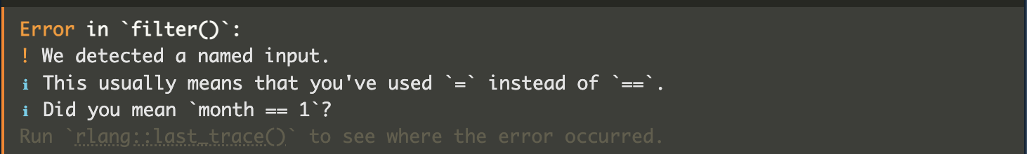
flights |> filter(month == 1)

# by multiple value
flights |> filter(month %in% c(1, 3))

# by negation
flights |> filter(month != 1)
flights |> filter(!month %in% c(1, 3))

# by multiple condition
flights |> filter(month == 1 & dep_delay > 120)
flights |> filter(month == 1, dep_delay > 120)
flights |> filter(month == 1 | dep_delay > 120)

Find all the entries with departure delay larger than 2 hours

What would flights |> filter(dep_delay > 120) do:

flights

# A tibble: 336,776 × 19
    year month   day dep_time sched_dep_time dep_delay
   <int> <int> <int>    <int>          <int>     <dbl>
 1  2013     1     1      517            515         2
 2  2013     1     1      533            529         4
 3  2013     1     1      542            540         2
 4  2013     1     1      544            545        -1
 5  2013     1     1      554            600        -6
 6  2013     1     1      554            558        -4
 7  2013     1     1      555            600        -5
 8  2013     1     1      557            600        -3
 9  2013     1     1      557            600        -3
10  2013     1     1      558            600        -2
# ℹ 336,766 more rows
# ℹ 13 more variables: arr_time <int>,
#   sched_arr_time <int>, arr_delay <dbl>, carrier <chr>,
#   flight <int>, tailnum <chr>, origin <chr>, dest <chr>,
#   air_time <dbl>, distance <dbl>, hour <dbl>,
#   minute <dbl>, time_hour <dttm>

Let’s check whether each departure delay is larger than 120 and only keep those that are TRUE.

# A tibble: 336,776 × 2
   dep_delay `dep_delay > 120`
       <dbl> <lgl>            
 1         2 FALSE            
 2         4 FALSE            
 3         2 FALSE            
 4        -1 FALSE            
 5        -6 FALSE            
 6        -4 FALSE            
 7        -5 FALSE            
 8        -3 FALSE            
 9        -3 FALSE            
10        -2 FALSE            
# ℹ 336,766 more rows

Find all the entries with departure delay larger than 2 hours

flights

# A tibble: 336,776 × 19
    year month   day dep_time sched_dep_time dep_delay
   <int> <int> <int>    <int>          <int>     <dbl>
 1  2013     1     1      517            515         2
 2  2013     1     1      533            529         4
 3  2013     1     1      542            540         2
 4  2013     1     1      544            545        -1
 5  2013     1     1      554            600        -6
 6  2013     1     1      554            558        -4
 7  2013     1     1      555            600        -5
 8  2013     1     1      557            600        -3
 9  2013     1     1      557            600        -3
10  2013     1     1      558            600        -2
# ℹ 336,766 more rows
# ℹ 13 more variables: arr_time <int>,
#   sched_arr_time <int>, arr_delay <dbl>, carrier <chr>,
#   flight <int>, tailnum <chr>, origin <chr>, dest <chr>,
#   air_time <dbl>, distance <dbl>, hour <dbl>,
#   minute <dbl>, time_hour <dttm>

flights |> filter(dep_delay > 120)

# A tibble: 9,723 × 19
    year month   day dep_time sched_dep_time dep_delay
   <int> <int> <int>    <int>          <int>     <dbl>
 1  2013     1     1      848           1835       853
 2  2013     1     1      957            733       144
 3  2013     1     1     1114            900       134
 4  2013     1     1     1540           1338       122
 5  2013     1     1     1815           1325       290
 6  2013     1     1     1842           1422       260
 7  2013     1     1     1856           1645       131
 8  2013     1     1     1934           1725       129
 9  2013     1     1     1938           1703       155
10  2013     1     1     1942           1705       157
# ℹ 9,713 more rows
# ℹ 13 more variables: arr_time <int>,
#   sched_arr_time <int>, arr_delay <dbl>, carrier <chr>,
#   flight <int>, tailnum <chr>, origin <chr>, dest <chr>,
#   air_time <dbl>, distance <dbl>, hour <dbl>,
#   minute <dbl>, time_hour <dttm>

Find all the entries in January

flights |> filter(month == 1)

# A tibble: 27,004 × 19
    year month   day dep_time sched_dep_time dep_delay arr_time sched_arr_time
   <int> <int> <int>    <int>          <int>     <dbl>    <int>          <int>
 1  2013     1     1      517            515         2      830            819
 2  2013     1     1      533            529         4      850            830
 3  2013     1     1      542            540         2      923            850
 4  2013     1     1      544            545        -1     1004           1022
 5  2013     1     1      554            600        -6      812            837
 6  2013     1     1      554            558        -4      740            728
 7  2013     1     1      555            600        -5      913            854
 8  2013     1     1      557            600        -3      709            723
 9  2013     1     1      557            600        -3      838            846
10  2013     1     1      558            600        -2      753            745
# ℹ 26,994 more rows
# ℹ 11 more variables: arr_delay <dbl>, carrier <chr>, flight <int>,
#   tailnum <chr>, origin <chr>, dest <chr>, air_time <dbl>, distance <dbl>,
#   hour <dbl>, minute <dbl>, time_hour <dttm>

What goes wrong here?

flights |> filter(month = 1)

flights |> filter(month == 1)

# A tibble: 27,004 × 19
    year month   day dep_time sched_dep_time dep_delay arr_time sched_arr_time
   <int> <int> <int>    <int>          <int>     <dbl>    <int>          <int>
 1  2013     1     1      517            515         2      830            819
 2  2013     1     1      533            529         4      850            830
 3  2013     1     1      542            540         2      923            850
 4  2013     1     1      544            545        -1     1004           1022
 5  2013     1     1      554            600        -6      812            837
 6  2013     1     1      554            558        -4      740            728
 7  2013     1     1      555            600        -5      913            854
 8  2013     1     1      557            600        -3      709            723
 9  2013     1     1      557            600        -3      838            846
10  2013     1     1      558            600        -2      753            745
# ℹ 26,994 more rows
# ℹ 11 more variables: arr_delay <dbl>, carrier <chr>, flight <int>,
#   tailnum <chr>, origin <chr>, dest <chr>, air_time <dbl>, distance <dbl>,
#   hour <dbl>, minute <dbl>, time_hour <dttm>

Your time

usethis::create_from_github("SDS322E-2025FALL/0203-dplyr")

Read slides 4 and 5 to write the code answering the following questions:

Find the flights that depart from JFK
Find the flights that depart from JFK in January
Find the flights that depart from EWR and LGA and not in January

You may start from:

flights |> filter(...)

Solution

Find the flights that depart from JFK

flights |> filter(origin == "JFK")

Find the flights that depart from JFK and LGA in January

flights |> filter(origin %in% c("JFK", "LGA"), month == 1)
# its also okay to write
flights |> filter(origin %in% c("JFK", "LGA") & month == 1)

Find the flights that not depart from EWR and LGA and not in January

flights |> filter(!origin %in% c("EWR", "LGA"), month != 1)

`mutate()` syntax

DATA |> mutate(VARIABLE = EXPRESSION)

If VARIABLE already exists, it modifies the column; otherwise, it will create a new one.

flights |> mutate(gain = dep_delay - arr_delay)

# A tibble: 336,776 × 20
    year month   day dep_time sched_dep_time dep_delay arr_time sched_arr_time
   <int> <int> <int>    <int>          <int>     <dbl>    <int>          <int>
 1  2013     1     1      517            515         2      830            819
 2  2013     1     1      533            529         4      850            830
 3  2013     1     1      542            540         2      923            850
 4  2013     1     1      544            545        -1     1004           1022
 5  2013     1     1      554            600        -6      812            837
 6  2013     1     1      554            558        -4      740            728
 7  2013     1     1      555            600        -5      913            854
 8  2013     1     1      557            600        -3      709            723
 9  2013     1     1      557            600        -3      838            846
10  2013     1     1      558            600        -2      753            745
# ℹ 336,766 more rows
# ℹ 12 more variables: arr_delay <dbl>, carrier <chr>, flight <int>,
#   tailnum <chr>, origin <chr>, dest <chr>, air_time <dbl>, distance <dbl>,
#   hour <dbl>, minute <dbl>, time_hour <dttm>, gain <dbl>

You can put multiple mutations together, or separately

These two are identical:

flights |> 
  mutate(gain = dep_delay - arr_delay, 
         speed = distance / (air_time / 60))

# A tibble: 336,776 × 21
    year month   day dep_time sched_dep_time
   <int> <int> <int>    <int>          <int>
 1  2013     1     1      517            515
 2  2013     1     1      533            529
 3  2013     1     1      542            540
 4  2013     1     1      544            545
 5  2013     1     1      554            600
 6  2013     1     1      554            558
 7  2013     1     1      555            600
 8  2013     1     1      557            600
 9  2013     1     1      557            600
10  2013     1     1      558            600
# ℹ 336,766 more rows
# ℹ 16 more variables: dep_delay <dbl>,
#   arr_time <int>, sched_arr_time <int>,
#   arr_delay <dbl>, carrier <chr>, flight <int>,
#   tailnum <chr>, origin <chr>, dest <chr>,
#   air_time <dbl>, distance <dbl>, hour <dbl>,
#   minute <dbl>, time_hour <dttm>, gain <dbl>, …

flights |> 
  mutate(gain = dep_delay - arr_delay) |> 
  mutate(speed = distance / (air_time / 60))

# A tibble: 336,776 × 21
    year month   day dep_time sched_dep_time
   <int> <int> <int>    <int>          <int>
 1  2013     1     1      517            515
 2  2013     1     1      533            529
 3  2013     1     1      542            540
 4  2013     1     1      544            545
 5  2013     1     1      554            600
 6  2013     1     1      554            558
 7  2013     1     1      555            600
 8  2013     1     1      557            600
 9  2013     1     1      557            600
10  2013     1     1      558            600
# ℹ 336,766 more rows
# ℹ 16 more variables: dep_delay <dbl>,
#   arr_time <int>, sched_arr_time <int>,
#   arr_delay <dbl>, carrier <chr>, flight <int>,
#   tailnum <chr>, origin <chr>, dest <chr>,
#   air_time <dbl>, distance <dbl>, hour <dbl>,
#   minute <dbl>, time_hour <dttm>, gain <dbl>, …

We can also compare them properly :)

v1 <- flights |> 
  mutate(gain = dep_delay - arr_delay, 
         speed = distance / (air_time / 60))

v2 <- flights |> 
  mutate(gain = dep_delay - arr_delay) |> 
  mutate(speed = distance / (air_time / 60))

identical(v1, v2)

[1] TRUE

Something about design

By default, columns are mutated in the end of the data frame, what if you want to put them at position xxxx? How do I do something like this?

# A tibble: 6 × 20
   gain  year month   day dep_time sched_dep_time dep_delay arr_time
  <dbl> <int> <int> <int>    <int>          <int>     <dbl>    <int>
1    -9  2013     1     1      517            515         2      830
2   -16  2013     1     1      533            529         4      850
3   -31  2013     1     1      542            540         2      923
4    17  2013     1     1      544            545        -1     1004
5    19  2013     1     1      554            600        -6      812
6   -16  2013     1     1      554            558        -4      740
# ℹ 12 more variables: sched_arr_time <int>, arr_delay <dbl>, carrier <chr>,
#   flight <int>, tailnum <chr>, origin <chr>, dest <chr>, air_time <dbl>,
#   distance <dbl>, hour <dbl>, minute <dbl>, time_hour <dttm>

Part of the reason tidyverse is neat is that it makes things easy. But define easy …

You will expect for every main task, you don’t need to do much for small tweaks.

Your time

Read the documentation of mutate() and modify the following code to put the gain column:

flights |> 
  mutate(gain = dep_delay - arr_delay)

as the first column,
after the day variable, and
keep only the columns used to create the gain column

Solution

flights |> mutate(gain = dep_delay - arr_delay, .before = 1) 
flights |> mutate(gain = dep_delay - arr_delay, .after = day)
flights |> mutate(gain = dep_delay - arr_delay, .keep = "used")

Why these arguments have “.” in front of everything?

Function developer needs to accommodate the fact that users will do all sorts of things with their functions, e.g. you may name a column after for the number of mins after the scheduled time
If after is also an argument name inside mutate(), it will then be confusing whether you are referring to the column or the argument.
Prefixing the argument name with . avoids this problem – it’s a good practice.

I don’t say you should prefix all your variables with ., but package developers should do that for good practice.

Sorry, Allison Horst doesn’t have art illustration for `group_by()` and `summarize()`

`group_by()` and `summarize()`

DATA |> group_by(VARIABLEs) |> summarize(EXPRESSION)

Example:

flights |> group_by(month)

# A tibble: 336,776 × 19
# Groups:   month [12]
    year month   day dep_time sched_dep_time dep_delay arr_time sched_arr_time
   <int> <int> <int>    <int>          <int>     <dbl>    <int>          <int>
 1  2013     1     1      517            515         2      830            819
 2  2013     1     1      533            529         4      850            830
 3  2013     1     1      542            540         2      923            850
 4  2013     1     1      544            545        -1     1004           1022
 5  2013     1     1      554            600        -6      812            837
 6  2013     1     1      554            558        -4      740            728
 7  2013     1     1      555            600        -5      913            854
 8  2013     1     1      557            600        -3      709            723
 9  2013     1     1      557            600        -3      838            846
10  2013     1     1      558            600        -2      753            745
# ℹ 336,766 more rows
# ℹ 11 more variables: arr_delay <dbl>, carrier <chr>, flight <int>,
#   tailnum <chr>, origin <chr>, dest <chr>, air_time <dbl>, distance <dbl>,
#   hour <dbl>, minute <dbl>, time_hour <dttm>

The header tells you that the data is grouped by month and there are 12 groups (12 months).

Example

Why we get all the NAs here?

flights |>
  group_by(month) |>
  summarize(avg_dep_delay = mean(dep_delay))

# A tibble: 12 × 2
   month avg_dep_delay
   <int>         <dbl>
 1     1            NA
 2     2            NA
 3     3            NA
 4     4            NA
 5     5            NA
 6     6            NA
 7     7            NA
 8     8            NA
 9     9            NA
10    10            NA
# ℹ 2 more rows

I hope you remember:

flights |>
  group_by(month) |>
  summarize(avg_dep_delay = 
              mean(dep_delay, na.rm = TRUE))

# A tibble: 12 × 2
   month avg_dep_delay
   <int>         <dbl>
 1     1         10.0 
 2     2         10.8 
 3     3         13.2 
 4     4         13.9 
 5     5         13.0 
 6     6         20.8 
 7     7         21.7 
 8     8         12.6 
 9     9          6.72
10    10          6.24
# ℹ 2 more rows

But notice `summarize()` and `summary()` are two different verbs

summarize() is a dplyr verb to summarize groups in a way you specified
summary() is a base R function to provide the 5 number summary (min, quantile, median, mean, max) for each variable in a data frame

summary(flights$dep_delay)

   Min. 1st Qu.  Median    Mean 3rd Qu.    Max.    NA's 
 -43.00   -5.00   -2.00   12.64   11.00 1301.00    8255

flights |>
  group_by(month) |>
  summarize(avg_dep_delay = 
              mean(dep_delay, na.rm = TRUE))

# A tibble: 12 × 2
   month avg_dep_delay
   <int>         <dbl>
 1     1         10.0 
 2     2         10.8 
 3     3         13.2 
 4     4         13.9 
 5     5         13.0 
 6     6         20.8 
 7     7         21.7 
 8     8         12.6 
 9     9          6.72
10    10          6.24
# ℹ 2 more rows

Of course, you can do multiple summaries

flights |>
  group_by(month, origin) |>
  summarize(avg_dep_delay = mean(dep_delay, na.rm = TRUE),
            avg_arr_delay = mean(arr_delay, na.rm = TRUE))

# A tibble: 36 × 4
# Groups:   month [12]
   month origin avg_dep_delay avg_arr_delay
   <int> <chr>          <dbl>         <dbl>
 1     1 EWR            14.9          12.8 
 2     1 JFK             8.62          1.37
 3     1 LGA             5.64          3.38
 4     2 EWR            13.1           8.78
 5     2 JFK            11.8           4.39
 6     2 LGA             6.96          3.15
 7     3 EWR            18.1          10.6 
 8     3 JFK            10.7           2.58
 9     3 LGA            10.2           3.74
10     4 EWR            17.4          14.1 
# ℹ 26 more rows

But the following means summarize avg_dep_delay first, then summarize avg_arr_delay from the result of the first summary, which is not what we want:

flights |>
  group_by(month, origin) |>
  summarize(avg_dep_delay = mean(dep_delay, na.rm = TRUE)) |> 
  summarize(avg_arr_delay = mean(arr_delay, na.rm = TRUE))

Your time

Apply the group_by() + summarize() syntax to calculate the average flight distance for each of the three origins. Your results should look like this:

# A tibble: 3 × 2
  origin distance
  <chr>     <dbl>
1 EWR       1057.
2 JFK       1266.
3 LGA        780.

Solution

flights |> group_by(origin) |> summarize(distance = mean(distance, na.rm = TRUE))

# A tibble: 3 × 2
  origin distance
  <chr>     <dbl>
1 EWR       1057.
2 JFK       1266.
3 LGA        780.

Let me sneak in a new verb: `arrange()`

Sometimes, we may wish to have the result sorted by a variable, this can be done with arrange():

flights |>
  group_by(carrier) |>
  summarize(avg_dep_delay = 
              mean(arr_delay, na.rm = TRUE))

# A tibble: 16 × 2
   carrier avg_dep_delay
   <chr>           <dbl>
 1 9E              7.38 
 2 AA              0.364
 3 AS             -9.93 
 4 B6              9.46 
 5 DL              1.64 
 6 EV             15.8  
 7 F9             21.9  
 8 FL             20.1  
 9 HA             -6.92 
10 MQ             10.8  
# ℹ 6 more rows

flights |>
  group_by(carrier) |>
  summarize(avg_dep_delay = 
              mean(arr_delay, na.rm = TRUE)) |> 
  arrange(avg_dep_delay)

# A tibble: 16 × 2
   carrier avg_dep_delay
   <chr>           <dbl>
 1 AS             -9.93 
 2 HA             -6.92 
 3 AA              0.364
 4 DL              1.64 
 5 VX              1.76 
 6 US              2.13 
 7 UA              3.56 
 8 9E              7.38 
 9 B6              9.46 
10 WN              9.65 
# ℹ 6 more rows

Let me sneak in a new verb: `arrange()`

Sort by decreasing order can be done with either - or desc():

flights |>
  group_by(carrier) |>
  summarize(avg_dep_delay = 
              mean(arr_delay, na.rm = TRUE)) |> 
  arrange(-avg_dep_delay)

# A tibble: 16 × 2
   carrier avg_dep_delay
   <chr>           <dbl>
 1 F9             21.9  
 2 FL             20.1  
 3 EV             15.8  
 4 YV             15.6  
 5 OO             11.9  
 6 MQ             10.8  
 7 WN              9.65 
 8 B6              9.46 
 9 9E              7.38 
10 UA              3.56 
11 US              2.13 
12 VX              1.76 
13 DL              1.64 
14 AA              0.364
15 HA             -6.92 
16 AS             -9.93

flights |>
  group_by(carrier) |>
  summarize(avg_dep_delay = 
              mean(arr_delay, na.rm = TRUE)) |> 
  arrange(desc(avg_dep_delay))

# A tibble: 16 × 2
   carrier avg_dep_delay
   <chr>           <dbl>
 1 F9             21.9  
 2 FL             20.1  
 3 EV             15.8  
 4 YV             15.6  
 5 OO             11.9  
 6 MQ             10.8  
 7 WN              9.65 
 8 B6              9.46 
 9 9E              7.38 
10 UA              3.56 
11 US              2.13 
12 VX              1.76 
13 DL              1.64 
14 AA              0.364
15 HA             -6.92 
16 AS             -9.93

Your time

Can you improve the previous group_by() and summarize() code to show the distance sorted from small to large as this:

# A tibble: 3 × 2
  origin distance
  <chr>     <dbl>
1 LGA        780.
2 EWR       1057.
3 JFK       1266.

Solution

flights |> 
  group_by(origin) |>
  summarize(distance = mean(distance, na.rm = TRUE)) |> 
  arrange(distance)

# A tibble: 3 × 2
  origin distance
  <chr>     <dbl>
1 LGA        780.
2 EWR       1057.
3 JFK       1266.

Combine everything together: Decompose a problem into dplyr verbs

Task: We want to summarize the proportion of flights with departure delay larger than 2 hours.

Thought process:

I need label the rows as whether they are delay more than 2 hrs or not.

This sounds like a mutate() and we learn the “larger than 2 hrs” part in filter()

flights |> 
  mutate(over_2h_delay = dep_delay > 120, .keep = "used")

# A tibble: 336,776 × 2
   dep_delay over_2h_delay
       <dbl> <lgl>        
 1         2 FALSE        
 2         4 FALSE        
 3         2 FALSE        
 4        -1 FALSE        
 5        -6 FALSE        
 6        -4 FALSE        
 7        -5 FALSE        
 8        -3 FALSE        
 9        -3 FALSE        
10        -2 FALSE        
11        -2 FALSE        
12        -2 FALSE        
13        -2 FALSE        
14        -2 FALSE        
15        -1 FALSE        
16         0 FALSE        
17        -1 FALSE        
18         0 FALSE        
19         0 FALSE        
20         1 FALSE        
# ℹ 336,756 more rows

Task: We want to summarize the proportion of flights with departure delay larger than 2 hours.

Thought process:

I need label the rows as whether they are delay more than 2 hrs or not.
Then I need to count the number of observations for over and below 2h delay.

This sounds like group_by() and summarize(), but I want what’s inside summarise() to be the count

flights |> 
  mutate(over_2h_delay = dep_delay > 120, .keep = "used") |> 
  group_by(over_2h_delay) |>
  summarise(n = n())

# A tibble: 3 × 2
  over_2h_delay      n
  <lgl>          <int>
1 FALSE         318798
2 TRUE            9723
3 NA              8255

Task: We want to summarize the proportion of flights with departure delay larger than 2 hours.

Thought process:

I need label the rows as whether they are delay more than 2 hrs or not.
Then I need to count the number of observations for over and below 2h delay.
Then I need to calculate proportion based on n.

This sounds like mutate() again

flights |> 
  mutate(over_2h_delay = dep_delay > 120, .keep = "used") |> 
  group_by(over_2h_delay) |>
  summarise(n = n()) |> 
  mutate(prop = n/ sum(n) * 100)

# A tibble: 3 × 3
  over_2h_delay      n  prop
  <lgl>          <int> <dbl>
1 FALSE         318798 94.7 
2 TRUE            9723  2.89
3 NA              8255  2.45

Remark 1

Can we look at those NAs?

flights |> filter(is.na(dep_delay))

# A tibble: 8,255 × 19
   year month   day dep_time sched_dep_time dep_delay
  <int> <int> <int>    <int>          <int>     <dbl>
1  2013     1     1       NA           1630        NA
2  2013     1     1       NA           1935        NA
3  2013     1     1       NA           1500        NA
4  2013     1     1       NA            600        NA
5  2013     1     2       NA           1540        NA
# ℹ 8,250 more rows
# ℹ 13 more variables: arr_time <int>,
#   sched_arr_time <int>, arr_delay <dbl>, carrier <chr>,
#   flight <int>, tailnum <chr>, origin <chr>, dest <chr>,
#   air_time <dbl>, distance <dbl>, hour <dbl>,
#   minute <dbl>, time_hour <dttm>

There are records with no arrival and departure time - we will need to keep them in mind about this data.

Why can’t you do

filter(dep_delay == NA)?

This is not legit because comparing anything with NA gives an NA (rather than giving FALSE):

1 == NA

[1] NA

2!= NA

[1] NA

Remark 2

group_by(over_2h_delay) |> summarise(n = n()) can be simplified with a single command dplyr::count(over_2h_delay).

flights |> 
  mutate(over_2h_delay = dep_delay > 120, 
         .keep = "used") |> 
  group_by(over_2h_delay) |>
  summarise(n = n()) |> 
  mutate(prop = n/ sum(n) * 100)

# A tibble: 3 × 3
  over_2h_delay      n  prop
  <lgl>          <int> <dbl>
1 FALSE         318798 94.7 
2 TRUE            9723  2.89
3 NA              8255  2.45

flights |> 
  mutate(over_2h_delay = dep_delay > 120, 
         .keep = "used") |> 
  count(over_2h_delay) |> 
  mutate(prop = n/ sum(n) * 100)

# A tibble: 3 × 3
  over_2h_delay      n  prop
  <lgl>          <int> <dbl>
1 FALSE         318798 94.7 
2 TRUE            9723  2.89
3 NA              8255  2.45

Your time

Can you reproduce the code we just walked through for the following task?

Task: We want to summarize the proportion of flights with departure delay larger than 2 hours.

Here is the step breakdown if you need:

I need label the rows as whether they are delay more than 2 hrs or not.
Then I need to count the number of observations for over and below 2h delay.
Then I need to calculate proportion based on n.

Elements of Data Science SDS 322E

Upcoming assessment

Seek helps during the office hours

Learning objective

dplyr syntax

dplyr syntax

dplyr syntax

dplyr syntax

Find all the entries with departure delay larger than 2 hours

Find all the entries with departure delay larger than 2 hours

Find all the entries in January

What goes wrong here?

Your time

Solution

mutate() syntax

You can put multiple mutations together, or separately

We can also compare them properly :)

Something about design

Your time

Solution

Sorry, Allison Horst doesn’t have art illustration for group_by() and summarize()

group_by() and summarize()

Example

But notice summarize() and summary() are two different verbs

Of course, you can do multiple summaries

Your time

Let me sneak in a new verb: arrange()

Let me sneak in a new verb: arrange()

Your time

Combine everything together: Decompose a problem into dplyr verbs

Remark 1

Remark 2

Your time

Elements of Data Science
SDS 322E

`dplyr` syntax

`dplyr` syntax

`dplyr` syntax

`dplyr` syntax

`mutate()` syntax

Sorry, Allison Horst doesn’t have art illustration for `group_by()` and `summarize()`

`group_by()` and `summarize()`

But notice `summarize()` and `summary()` are two different verbs

Let me sneak in a new verb: `arrange()`

Let me sneak in a new verb: `arrange()`