Elements of Data Science
SDS 322E

H. Sherry Zhang
Department of Statistics and Data Sciences
The University of Texas at Austin

Fall 2025

R history and ecosystem

• 1976: S was initiated as an internal statistical analysis environment—originally implemented as Fortran libraries. S is a language that was developed by John Chambers and others at Bell Labs.

• 1991: Created in New Zealand by Ross Ihaka and Robert Gentleman. Their experience developing R is documented in a 1996 JCGS paper.

• 1997: The R Core Group is formed (containing some people associated with S-PLUS). The core group controls the source code for R. See more about the Foundation: https://www.r-project.org/foundation/

Why R?

R code:

library(tidyverse)
mtcars |>
  mutate(kpl = mpg * 0.425144) |>
  filter(vs == 0) |>
  group_by(cyl) |>
  summarize(
    disp = mean(disp, na.rm = TRUE),
    kpl = mean(kpl, na.rm = TRUE)) |> 
  arrange(disp)

How would the FORTRAN 90 code look like?

FORTRAN 90 code for the same task

9 lines of code in R vs. 70 lines of code in FORTRAN 90

program mtcars_summary
    implicit none
    integer, parameter :: dp = selected_real_kind(15, 307)
    integer, parameter :: nmax = 100
    real(dp) :: mpg(nmax), disp(nmax), kpl(nmax)
    integer :: cyl(nmax), vs(nmax)
    integer :: i, n, j, ngrp, idx
    integer :: cyl_group(nmax)
    real(dp) :: disp_sum(nmax), kpl_sum(nmax)
    integer :: count(nmax)
    real(dp) :: disp_mean(nmax), kpl_mean(nmax)
    integer :: temp_i
    real(dp) :: temp_r
    ! open and read data
    open(unit=10, file='mtcars.csv', status='old', action='read')
    n = 0
    do
        read(10, *, end=100) mpg(n+1), cyl(n+1), disp(n+1), &
                              temp_r, temp_r, temp_r, temp_r, vs(n+1), &
                              temp_i, temp_i, temp_i
        n = n + 1
    end do
100 close(10)
    ! compute kpl
    do i = 1, n
        kpl(i) = mpg(i) * 0.425144_dp
    end do
    ! filter vs == 0
    ngrp = 0
    do i = 1, n
        if (vs(i) == 0) then
            ! check if cyl group already exists
            idx = 0
            do j = 1, ngrp
                if (cyl_group(j) == cyl(i)) idx = j
            end do
            if (idx == 0) then
                ngrp = ngrp + 1
                cyl_group(ngrp) = cyl(i)
                disp_sum(ngrp) = disp(i)
                kpl_sum(ngrp) = kpl(i)
                count(ngrp) = 1
            else
                disp_sum(idx) = disp_sum(idx) + disp(i)
                kpl_sum(idx)  = kpl_sum(idx) + kpl(i)
                count(idx)    = count(idx) + 1
            end if
        end if
    end do
    ! compute means
    do j = 1, ngrp
        disp_mean(j) = disp_sum(j) / count(j)
        kpl_mean(j)  = kpl_sum(j) / count(j)
    end do
    ! sort by disp_mean
    do i = 1, ngrp-1
        do j = i+1, ngrp
            if (disp_mean(j) < disp_mean(i)) then
                temp_r = disp_mean(i); disp_mean(i) = disp_mean(j); disp_mean(j) = temp_r
                temp_r = kpl_mean(i);  kpl_mean(i)  = kpl_mean(j);  kpl_mean(j)  = temp_r
                temp_i = cyl_group(i); cyl_group(i) = cyl_group(j); cyl_group(j) = temp_i
            end if
        end do
    end do
    ! print result
    print '(A4,2X,A10,2X,A10)', 'cyl', 'disp_mean', 'kpl_mean'
    do j = 1, ngrp
        print '(I4,2X,F10.3,2X,F10.3)', cyl_group(j), disp_mean(j), kpl_mean(j)
    end do
end program mtcars_summary

R ecosystem

• Base packages: base, methods, datasets, utils, grDevices, graphics, stats

• Recommended packages: MASS, lattice, Matrix, nlme, survival, boot, cluster, codetools, foreign, KernSmooth, rpart, spatial, splines, tcltk

• Contributed packages: 20,000 + packages contributed by users available on CRAN or Bioconductor (tidyverse lives here!) and more on GitHub (like emo).

The big picture

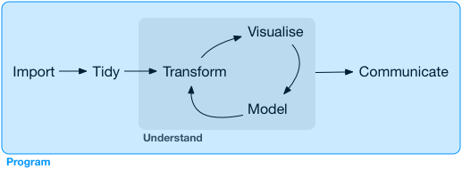
Transform (wrangling) - Week 2 - 3

You shall be able to do this for later assessment!

library(tidyverse)
mtcars |> 
  # create a new variable 
  mutate(kpl = mpg * 0.425144) |> 
  # "select" rows
  filter(vs == 0) |>
  # do things by groups
  group_by(cyl) |>  
  # create a data summarization
  summarize(disp = mean(disp, na.rm = TRUE), 
            kpl = mean(kpl, na.rm = TRUE)) |> 
  # sort the data frame by a variable
  arrange(disp)

Visualization - Week 3 - 4

You shall be able to do this for later assessment!

mtcars2 <- mtcars |> 
  mutate(vs = ifelse(vs == 0, "V-shaped", "Straight")) |>
  rename(Engine = vs) 

mtcars2 |> 
  ggplot(aes(x = mpg, y = disp, color = as.factor(cyl))) + 
  geom_point() + 
  facet_wrap(vars(Engine), labeller = label_both) + 
  scale_color_brewer(palette = "Dark2", name = "Number of cylinders") +
  theme_bw() + 
  theme(legend.position = "bottom") + 
  xlab("Miles per gallon") + 
  ylab("Displacement (cu.in.)")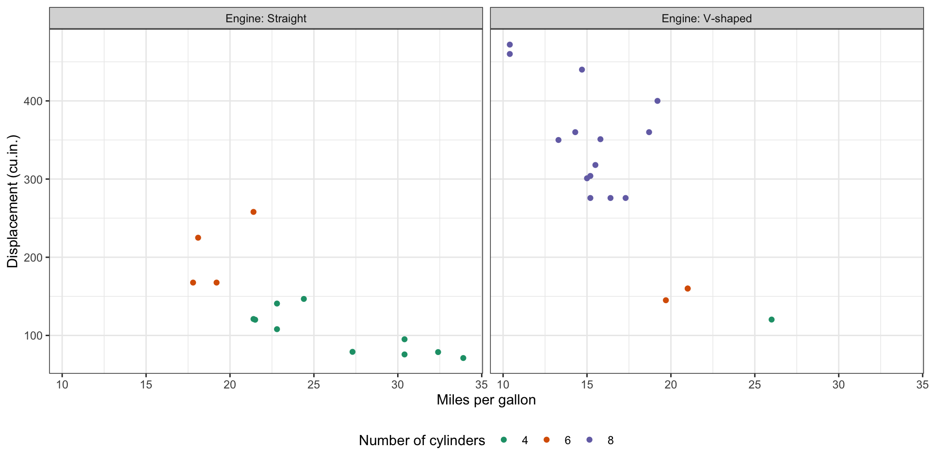

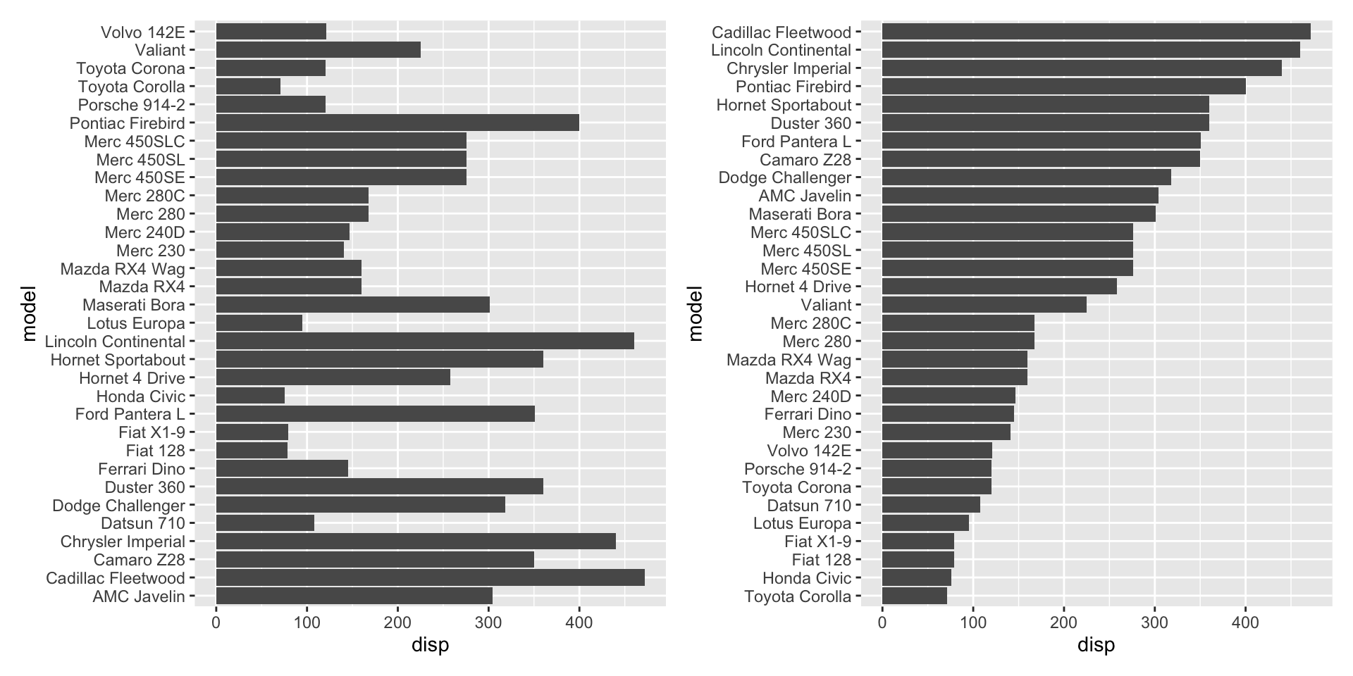
Visualization - week 3 - 4

Visual principles

In next few weeks…

Week	Date	Content
Week 2	09/03	Welcome to tidyverse, tidy data concept
	09/05	The dplyr package: mutate, select, filter, arrange, summarize
Week 3	09/08	More on dplyr verbs: pull, select, rename, between, ifelse, case_when
	09/10	Visualization with ggplot2: geometry + aesthetics
	09/12	Visualization with ggplot2: geometry + aesthetics
Week 4	09/15	Visualization with ggplot2: scale + color + facet + theme
	09/17	Advanced data wrangling: dplyr::*_join, tidyr::pivot_longer, and tidyr::pivot_wider
…		…

In next few weeks…

Week	Date	Content
Week 5	09/22	Spatial data: sf and ggplot2::geom_sf()
	09/24	Case study: flight data with map
	09/26	Let’s make animation and interactive graphics in R
Week 6	09/29	Case study: flight data - departure and arrival pattern
	10/01	Webscraping
	10/03	Case study: Wikipedia number of annual leave
Week 7	10/06	Wrangling string with stringr
	10/08	Text analysis with tidytext
	10/10	Project #1
Week 8	10/13	Sentiment analysis with tidytext
	10/15	Functional programming

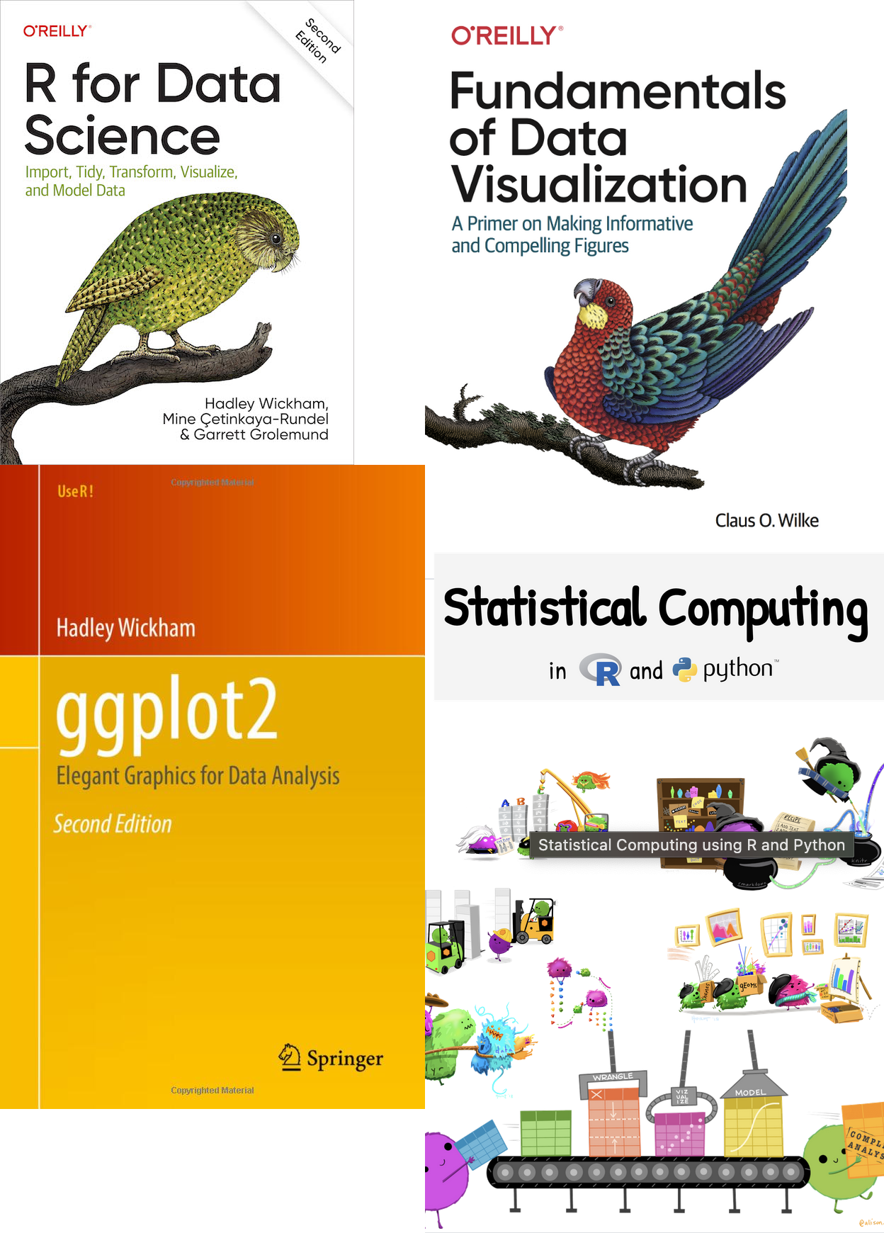
Resources

• R for Data Science by Hadley Wickham, Mine Çetinkaya-Rundel, and Garrett Grolemund: https://r4ds.hadley.nz/
• ggplot2: Elegant Graphics for Data Analysis (3e) by Hadley Wickham, Danielle Navarro, and Thomas Lin Pedersen: https://ggplot2-book.org/
• Fundamentals of Data Visualization by Claus O. Wilke: https://clauswilke.com/dataviz/
• Statistical Computing using R and Python by Susan Vanderplas: https://srvanderplas.github.io/stat-computing-r-python/

We will not learn Python in this course.

R basics

Gapminder Data

https://www.youtube.com/watch?v=jbkSRLYSojo&ab_channel=BBC

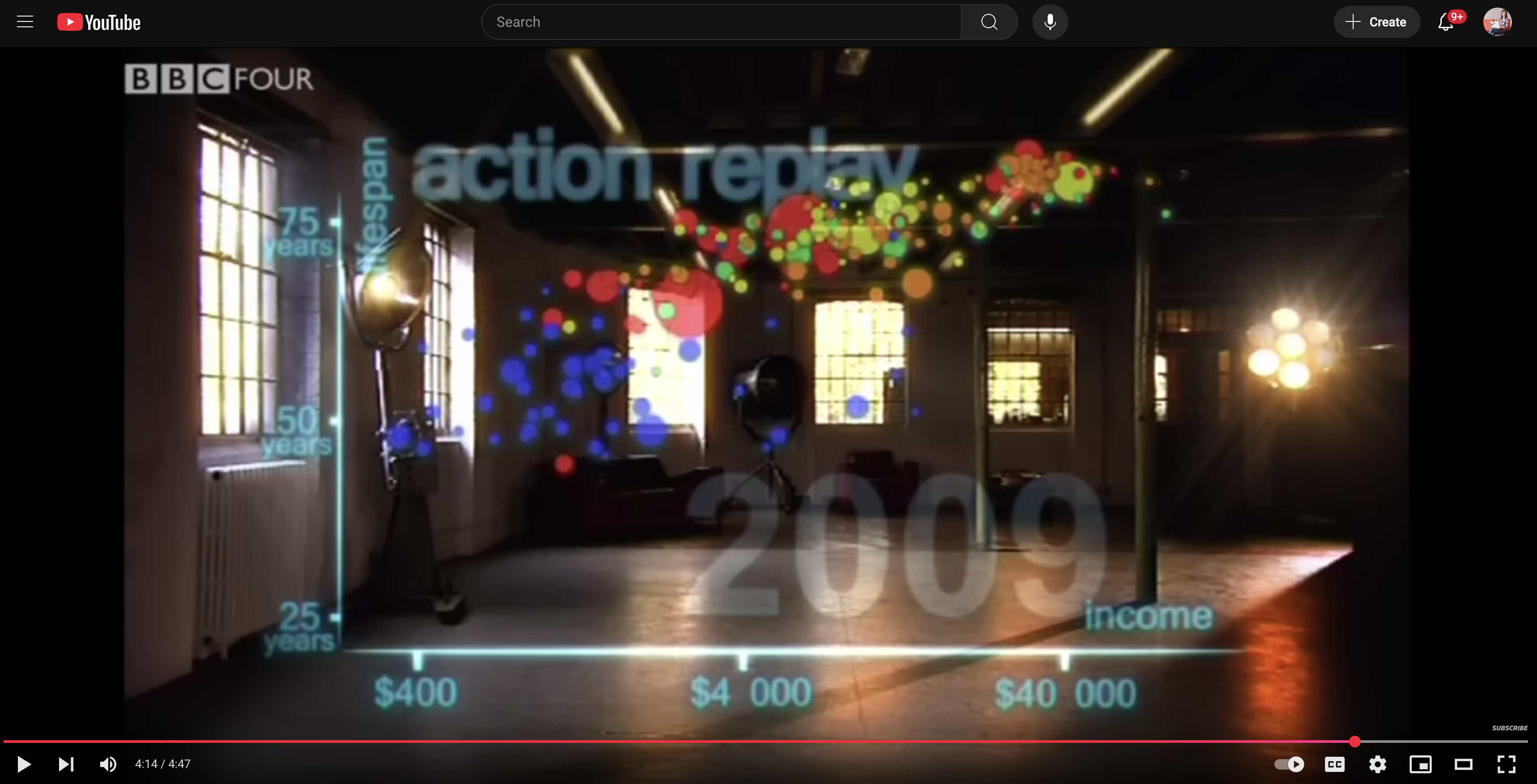
Gapminder Data

# install.packages("gapminder")
library(gapminder)
gapminder

# A tibble: 1,704 × 6
   country     continent  year lifeExp      pop gdpPercap
   <fct>       <fct>     <int>   <dbl>    <int>     <dbl>
 1 Afghanistan Asia       1952    28.8  8425333      779.
 2 Afghanistan Asia       1957    30.3  9240934      821.
 3 Afghanistan Asia       1962    32.0 10267083      853.
 4 Afghanistan Asia       1967    34.0 11537966      836.
 5 Afghanistan Asia       1972    36.1 13079460      740.
 6 Afghanistan Asia       1977    38.4 14880372      786.
 7 Afghanistan Asia       1982    39.9 12881816      978.
 8 Afghanistan Asia       1987    40.8 13867957      852.
 9 Afghanistan Asia       1992    41.7 16317921      649.
10 Afghanistan Asia       1997    41.8 22227415      635.
# ℹ 1,694 more rows

Read documentation

?gapminder

We can write some simple code to check the information in the documentation.

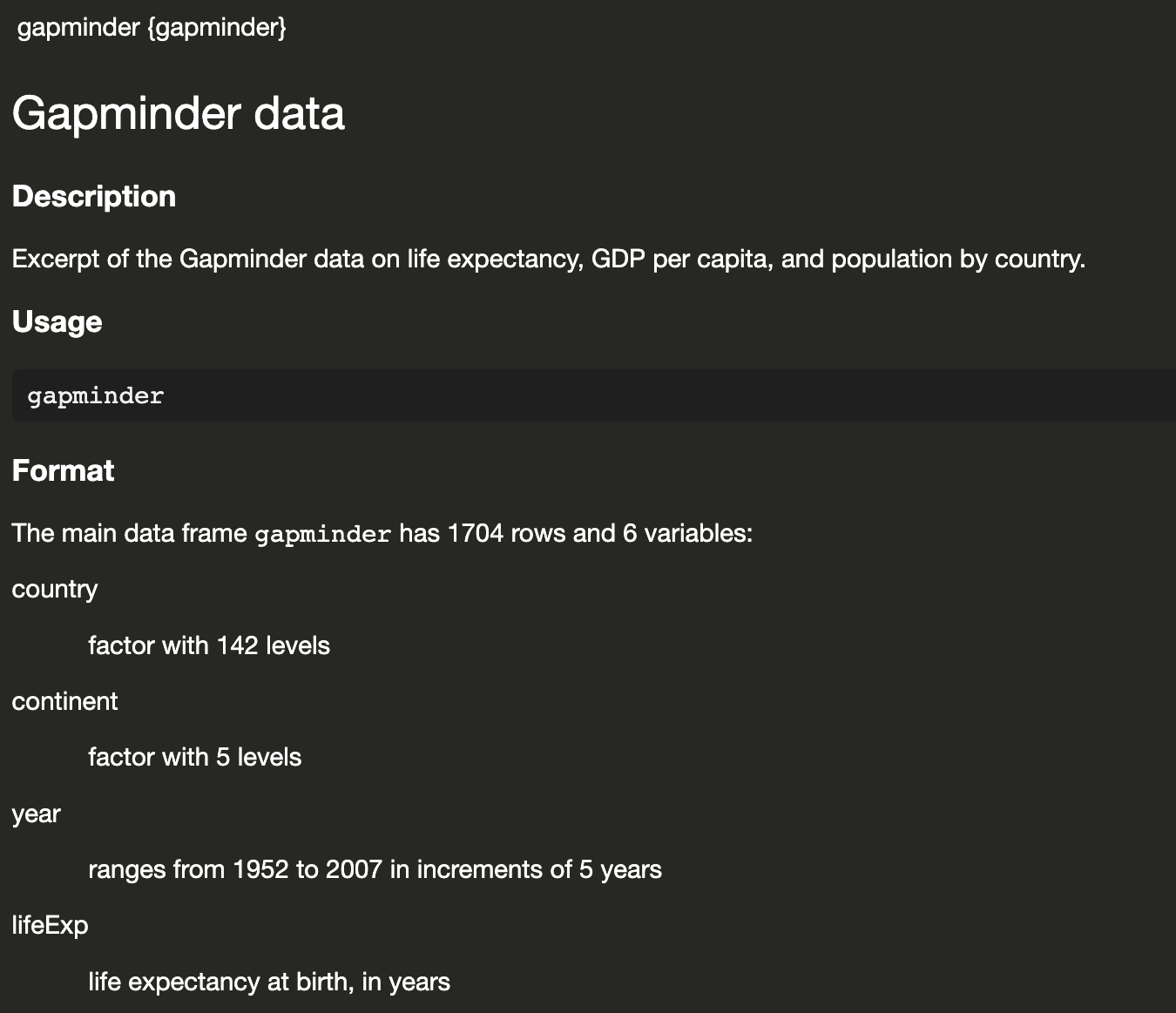
How many rows and how many columns?

The main data frame gapminder has 1704 rows and 6 variables:

nrow(gapminder)

[1] 1704

ncol(gapminder)

[1] 6

colnames(gapminder)

[1] "country"   "continent" "year"      "lifeExp"   "pop"       "gdpPercap"

Did you notice?

When we print the data, the header already tells you the number of rows and columns

#A tibble: 1,704 × 6

gapminder

# A tibble: 1,704 × 6
   country     continent  year lifeExp      pop gdpPercap
   <fct>       <fct>     <int>   <dbl>    <int>     <dbl>
 1 Afghanistan Asia       1952    28.8  8425333      779.
 2 Afghanistan Asia       1957    30.3  9240934      821.
 3 Afghanistan Asia       1962    32.0 10267083      853.
 4 Afghanistan Asia       1967    34.0 11537966      836.
 5 Afghanistan Asia       1972    36.1 13079460      740.
 6 Afghanistan Asia       1977    38.4 14880372      786.
 7 Afghanistan Asia       1982    39.9 12881816      978.
 8 Afghanistan Asia       1987    40.8 13867957      852.
 9 Afghanistan Asia       1992    41.7 16317921      649.
10 Afghanistan Asia       1997    41.8 22227415      635.
# ℹ 1,694 more rows

How many continent?

Continent is a factor with 5 levels

unique(gapminder$continent) 

[1] Asia     Europe   Africa   Americas Oceania 
Levels: Africa Americas Asia Europe Oceania

How many countries?

Country is a factor with 142 levels

unique(gapminder$country) 

  [1] Afghanistan              Albania                  Algeria                 
  [4] Angola                   Argentina                Australia               
  [7] Austria                  Bahrain                  Bangladesh              
 [10] Belgium                  Benin                    Bolivia                 
 [13] Bosnia and Herzegovina   Botswana                 Brazil                  
 [16] Bulgaria                 Burkina Faso             Burundi                 
 [19] Cambodia                 Cameroon                 Canada                  
 [22] Central African Republic Chad                     Chile                   
 [25] China                    Colombia                 Comoros                 
 [28] Congo, Dem. Rep.         Congo, Rep.              Costa Rica              
 [31] Cote d'Ivoire            Croatia                  Cuba                    
 [34] Czech Republic           Denmark                  Djibouti                
 [37] Dominican Republic       Ecuador                  Egypt                   
 [40] El Salvador              Equatorial Guinea        Eritrea                 
 [43] Ethiopia                 Finland                  France                  
 [46] Gabon                    Gambia                   Germany                 
 [49] Ghana                    Greece                   Guatemala               
 [52] Guinea                   Guinea-Bissau            Haiti                   
 [55] Honduras                 Hong Kong, China         Hungary                 
 [58] Iceland                  India                    Indonesia               
 [61] Iran                     Iraq                     Ireland                 
 [64] Israel                   Italy                    Jamaica                 
 [67] Japan                    Jordan                   Kenya                   
 [70] Korea, Dem. Rep.         Korea, Rep.              Kuwait                  
 [73] Lebanon                  Lesotho                  Liberia                 
 [76] Libya                    Madagascar               Malawi                  
 [79] Malaysia                 Mali                     Mauritania              
 [82] Mauritius                Mexico                   Mongolia                
 [85] Montenegro               Morocco                  Mozambique              
 [88] Myanmar                  Namibia                  Nepal                   
 [91] Netherlands              New Zealand              Nicaragua               
 [94] Niger                    Nigeria                  Norway                  
 [97] Oman                     Pakistan                 Panama                  
[100] Paraguay                 Peru                     Philippines             
[103] Poland                   Portugal                 Puerto Rico             
[106] Reunion                  Romania                  Rwanda                  
[109] Sao Tome and Principe    Saudi Arabia             Senegal                 
[112] Serbia                   Sierra Leone             Singapore               
[115] Slovak Republic          Slovenia                 Somalia                 
[118] South Africa             Spain                    Sri Lanka               
[121] Sudan                    Swaziland                Sweden                  
[124] Switzerland              Syria                    Taiwan                  
[127] Tanzania                 Thailand                 Togo                    
[130] Trinidad and Tobago      Tunisia                  Turkey                  
[133] Uganda                   United Kingdom           United States           
[136] Uruguay                  Venezuela                Vietnam                 
[139] West Bank and Gaza       Yemen, Rep.              Zambia                  
[142] Zimbabwe                
142 Levels: Afghanistan Albania Algeria Angola Argentina Australia ... Zimbabwe

How many countries?

Country is a factor with 142 levels

length(unique(gapminder$country))

[1] 142

What’ the range of year reported?

Year ranges from 1952 to 2007 in increments of 5 years

range(gapminder$year)

[1] 1952 2007

unique(gapminder$year)

 [1] 1952 1957 1962 1967 1972 1977 1982 1987 1992 1997 2002 2007

diff(unique(gapminder$year))

 [1] 5 5 5 5 5 5 5 5 5 5 5

What’s the min, mean, median, max of lifeExp?

min(gapminder$lifeExp)

[1] 23.599

mean(gapminder$lifeExp)

[1] 59.47444

median(gapminder$lifeExp)

[1] 60.7125

max(gapminder$lifeExp)

[1] 82.603

summary(gapminder$lifeExp)

   Min. 1st Qu.  Median    Mean 3rd Qu.    Max. 
  23.60   48.20   60.71   59.47   70.85   82.60 

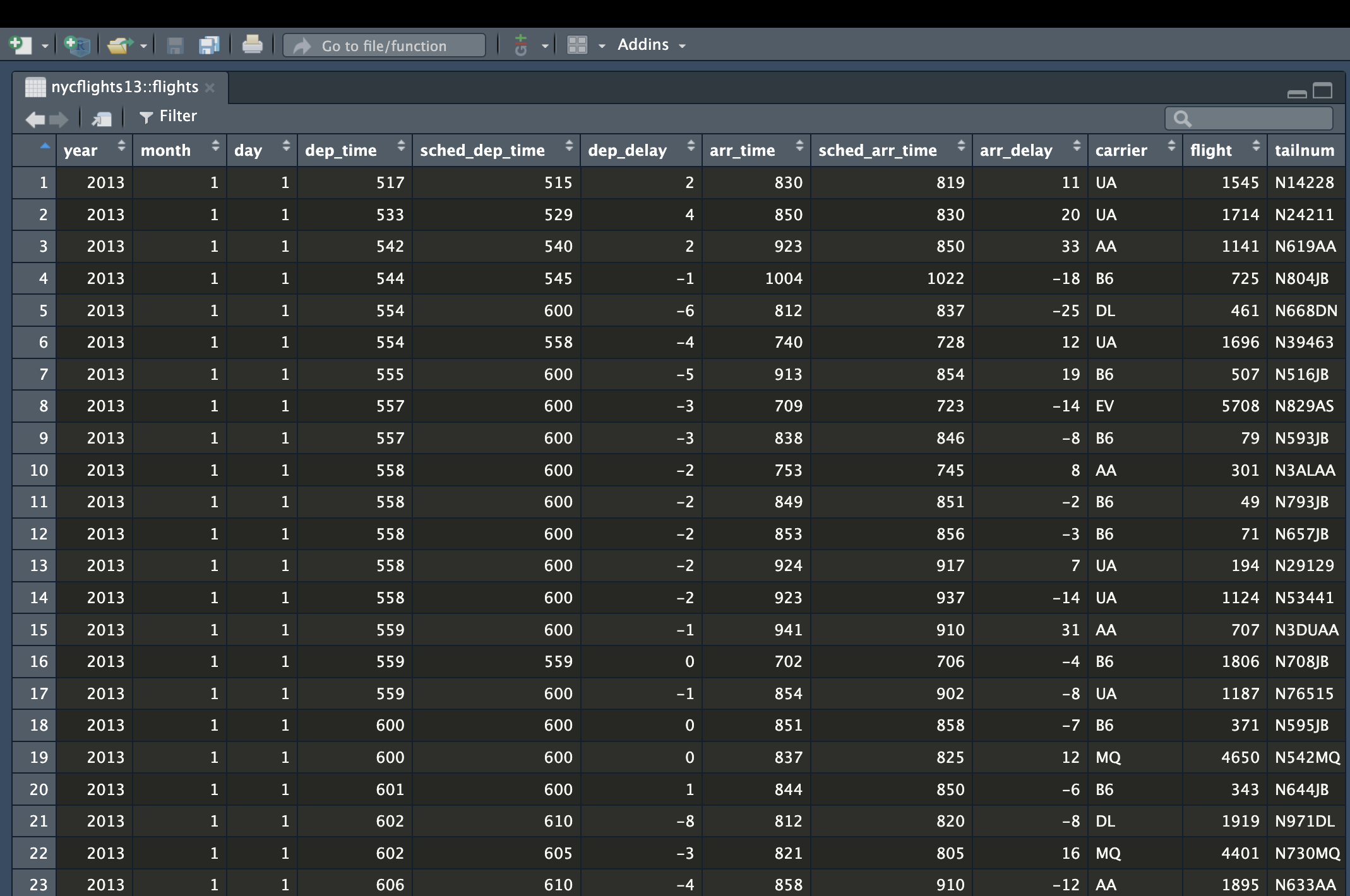
Flight data

library(nycflights13)
flights

# A tibble: 336,776 × 19
   year month   day dep_time sched_dep_time dep_delay arr_time sched_arr_time
  <int> <int> <int>    <int>          <int>     <dbl>    <int>          <int>
1  2013     1     1      517            515         2      830            819
2  2013     1     1      533            529         4      850            830
3  2013     1     1      542            540         2      923            850
4  2013     1     1      544            545        -1     1004           1022
5  2013     1     1      554            600        -6      812            837
# ℹ 336,771 more rows
# ℹ 11 more variables: arr_delay <dbl>, carrier <chr>, flight <int>,
#   tailnum <chr>, origin <chr>, dest <chr>, air_time <dbl>, distance <dbl>,
#   hour <dbl>, minute <dbl>, time_hour <dttm>

We can’t see all the variables - we need a better way to see it

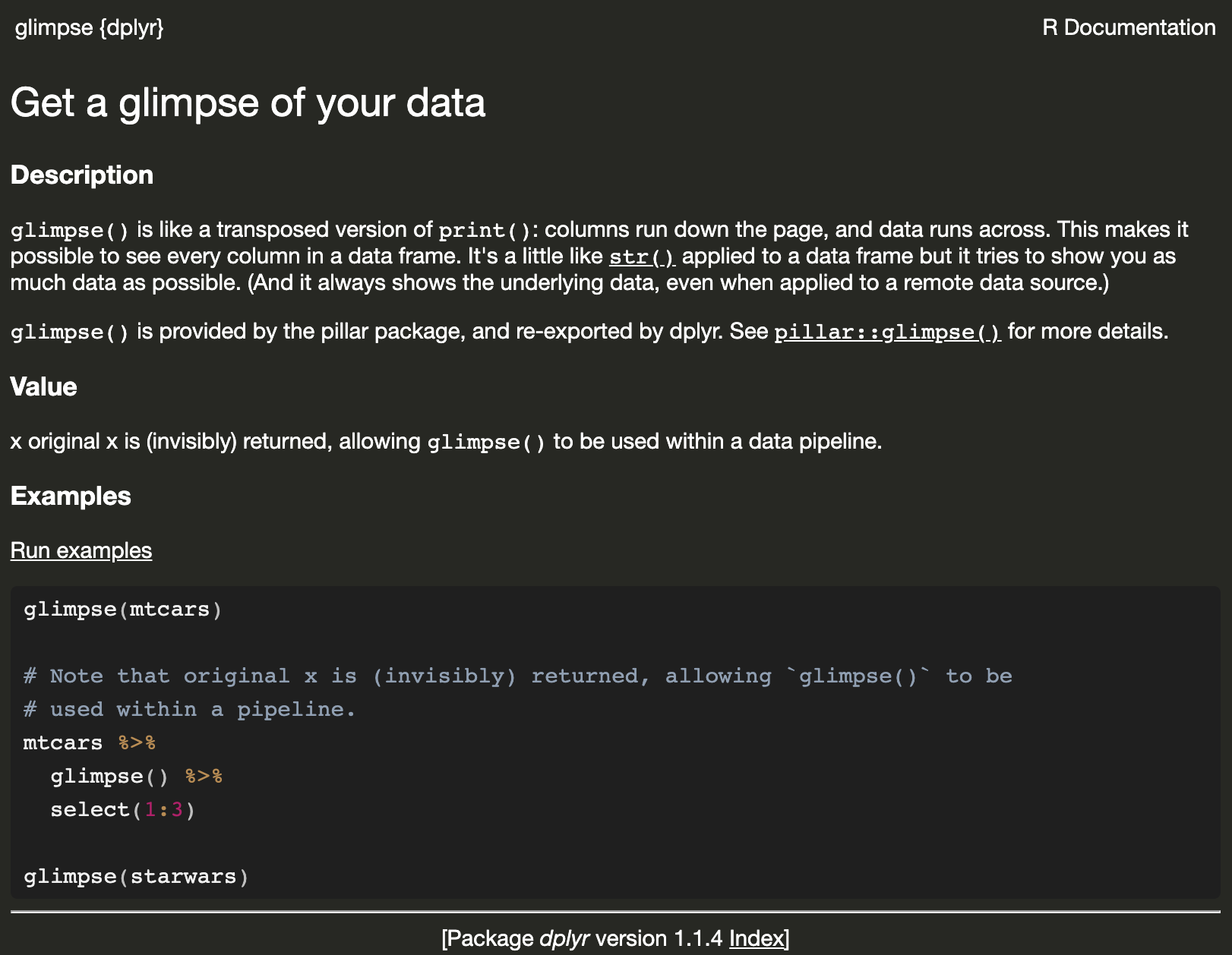
Flight data: dplyr::glimpse()

glimpse(flights)

Rows: 336,776
Columns: 19
$ year           <int> 2013, 2013, 2013, 2013, 2013, 2013,…
$ month          <int> 1, 1, 1, 1, 1, 1, 1, 1, 1, 1, 1, 1,…
$ day            <int> 1, 1, 1, 1, 1, 1, 1, 1, 1, 1, 1, 1,…
$ dep_time       <int> 517, 533, 542, 544, 554, 554, 555, …
$ sched_dep_time <int> 515, 529, 540, 545, 600, 558, 600, …
$ dep_delay      <dbl> 2, 4, 2, -1, -6, -4, -5, -3, -3, -2…
$ arr_time       <int> 830, 850, 923, 1004, 812, 740, 913,…
$ sched_arr_time <int> 819, 830, 850, 1022, 837, 728, 854,…
$ arr_delay      <dbl> 11, 20, 33, -18, -25, 12, 19, -14, …
$ carrier        <chr> "UA", "UA", "AA", "B6", "DL", "UA",…
$ flight         <int> 1545, 1714, 1141, 725, 461, 1696, 5…
$ tailnum        <chr> "N14228", "N24211", "N619AA", "N804…
$ origin         <chr> "EWR", "LGA", "JFK", "JFK", "LGA", …
$ dest           <chr> "IAH", "IAH", "MIA", "BQN", "ATL", …
$ air_time       <dbl> 227, 227, 160, 183, 116, 150, 158, …
$ distance       <dbl> 1400, 1416, 1089, 1576, 762, 719, 1…
$ hour           <dbl> 5, 5, 5, 5, 6, 5, 6, 6, 6, 6, 6, 6,…
$ minute         <dbl> 15, 29, 40, 45, 0, 58, 0, 0, 0, 0, …
$ time_hour      <dttm> 2013-01-01 05:00:00, 2013-01-01 05…

Access the documentation with ?

?dplyr::glimpse

Look at the first few rows

head(flights, n = 3)

# A tibble: 3 × 19
   year month   day dep_time sched_dep_time dep_delay
  <int> <int> <int>    <int>          <int>     <dbl>
1  2013     1     1      517            515         2
2  2013     1     1      533            529         4
3  2013     1     1      542            540         2
# ℹ 13 more variables: arr_time <int>,
#   sched_arr_time <int>, arr_delay <dbl>, carrier <chr>,
#   flight <int>, tailnum <chr>, origin <chr>, dest <chr>,
#   air_time <dbl>, distance <dbl>, hour <dbl>,
#   minute <dbl>, time_hour <dttm>

The last few rows?

tail(flights, n = 3)

# A tibble: 3 × 19
   year month   day dep_time sched_dep_time dep_delay
  <int> <int> <int>    <int>          <int>     <dbl>
1  2013     9    30       NA           1210        NA
2  2013     9    30       NA           1159        NA
3  2013     9    30       NA            840        NA
# ℹ 13 more variables: arr_time <int>,
#   sched_arr_time <int>, arr_delay <dbl>, carrier <chr>,
#   flight <int>, tailnum <chr>, origin <chr>, dest <chr>,
#   air_time <dbl>, distance <dbl>, hour <dbl>,
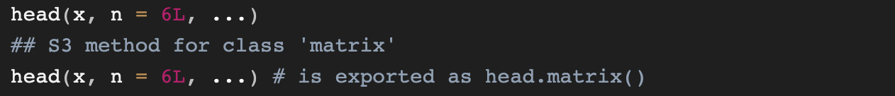
#   minute <dbl>, time_hour <dttm>

Check the documentation to see the default n value for head() and tail().

You can also View() the data

View(flights)

What’s the average of arrival delay (arr_delay)

mean(flights$arr_delay)

[1] NA

why?

tail(flights$arr_delay, n = 10)

 [1] -20 -16   1 -25  NA  NA  NA  NA  NA  NA

is.na(tail(flights$arr_delay, n = 10))

 [1] FALSE FALSE FALSE FALSE  TRUE  TRUE  TRUE  TRUE  TRUE  TRUE

A better way:

mean(flights$arr_delay, na.rm = TRUE)

[1] 6.895377

Lesson learnt

• Practice installing and loading packages with install.packages("pkg") and library(pkg).

• Read documentation of a function or a dataset with ?FUN or ?DATASET.

• Check the number of rows, columns, column names with nrow(), ncol(), colnames().

• Compute summary statistics with unique(), length(), range(), diff(), min(), mean(), median(), max(), summary(). Use the argument na.rm = TRUE to accommodate missing values.

• View data with View(), dplyr::glimpse() and View the first or last few rows with head() and tail().

Your time

Practice what we’ve just learn via

usethis::create_from_github("SDS322E-2025FALL/0103-basics", fork = FALSE)