H. Sherry Zhang Department of Statistics and Data Sciences University of Texas at Austin
Get the repository for today: library(usethis) create_from_github("SDS322E-26FALL/1202-trees", fork = FALSE)
Learning objectives
Understand the basic idea of decision trees for regression and classification
Fit decision trees using tidymodels for both regression and classification tasks
Identify the key parameters of decision trees and their effects
Understand the idea of random forest and how it improves over decision trees
Apply random forest using tidymodels (with hyper-parameter tuning)
Decision trees
Classification tree
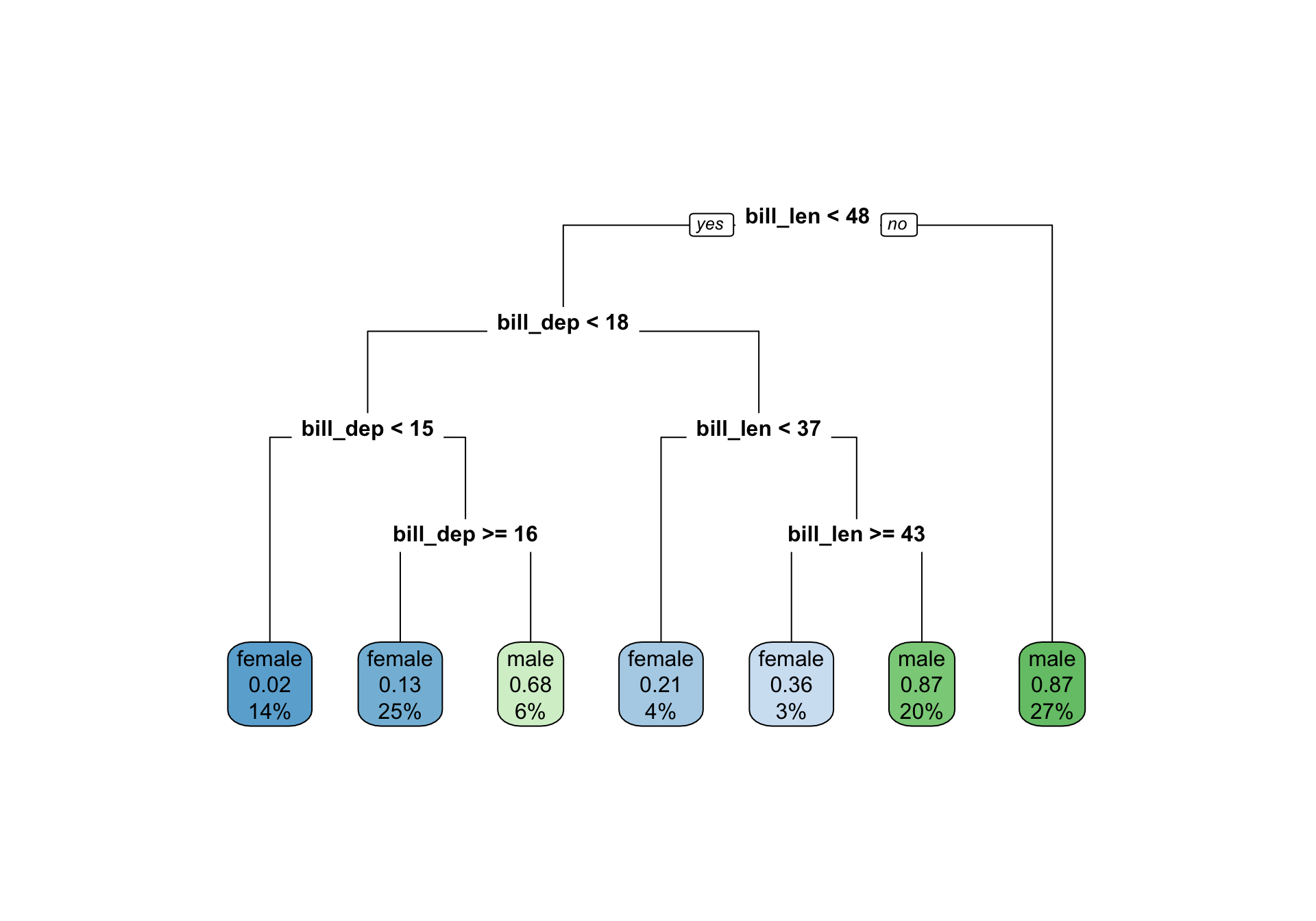
Can we predict penguin sex from bill_len and bill_dep with a few simple rules?
A tree is a set of yes/no questions. Start at the top and follow the answers down:
Is bill_len < 48? No (right): predict male
Yes (left): is bill_dep < 18? …
Each leaf at the bottom is a prediction: the majority class of the training penguins that end up there.
Classification tree
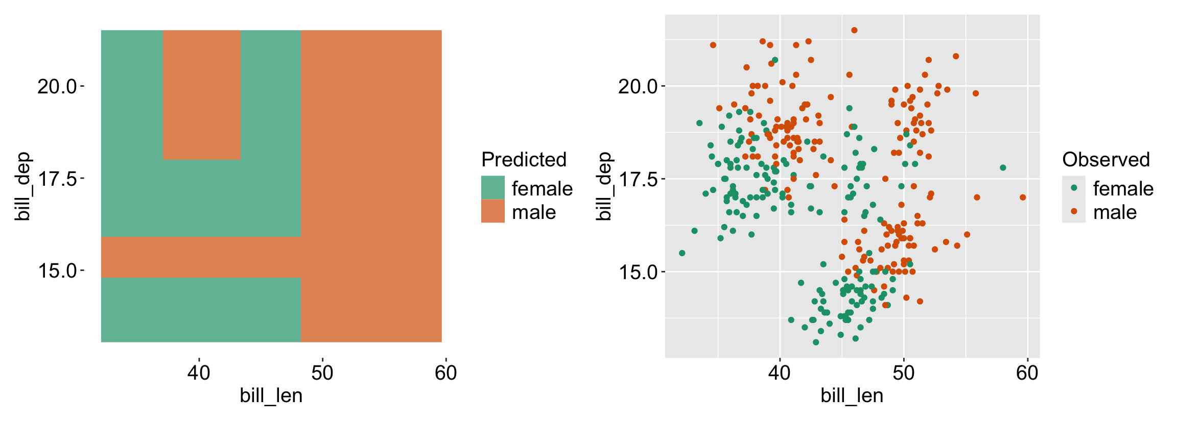
Divide/partition the predictor space \(X_1, \ldots, X_p\) into \(J\) regions \(R_1, \ldots, R_J\).
For every observation that falls within region \(R_j\), we make the same prediction: the majority class of the training observations in \(R_j\).
The goal is to increase the “purity” of each region, so that most regions are dominated by a single class: choose the splits that minimize the impurity (Gini index or entropy, see the appendix).
Each rectangle is one leaf of the tree: the splits are always parallel to the axes.
Regression tree
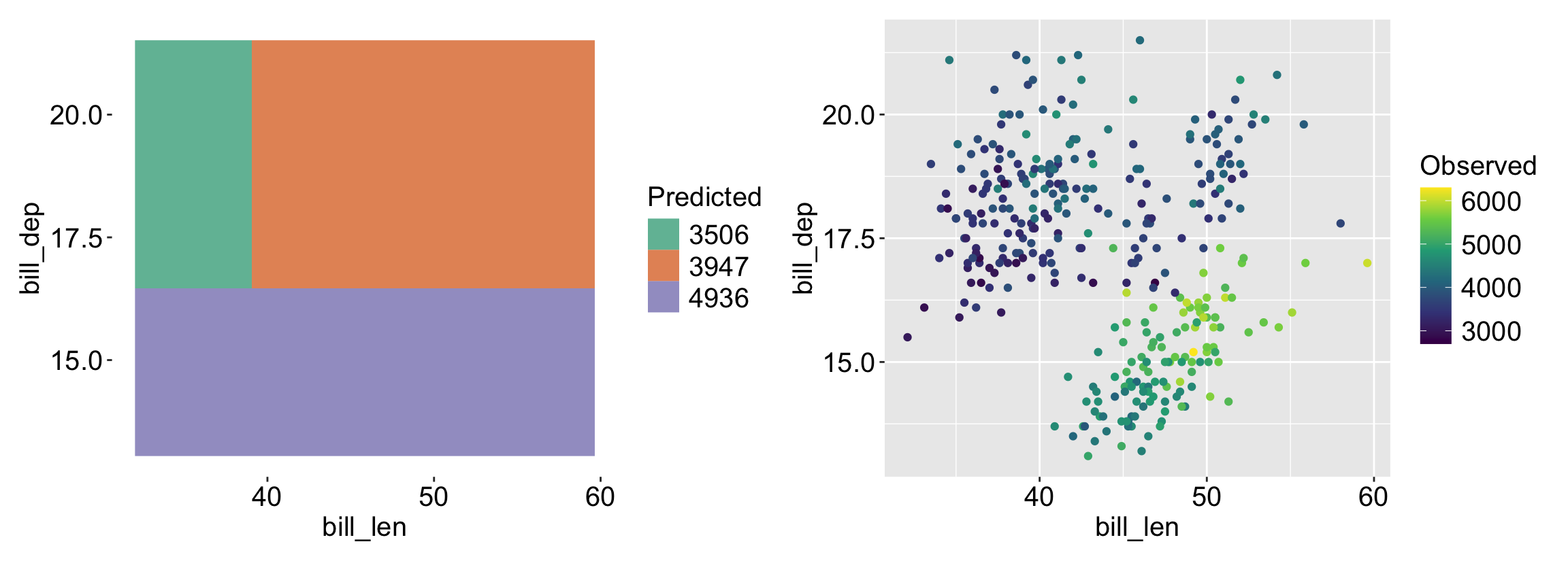
The same partition of the predictor space into regions \(R_1, \ldots, R_J\), but the response is now numeric.
For every observation that falls within region \(R_j\), we predict \(\bar{y}_{R_j}\): the mean of the response values for the training observations in \(R_j\) (instead of the majority class).
Purity doesn’t apply to a numeric response, so we choose the splits that minimize the residual sum of squares instead: \(RSS = \sum_{j=1}^{J} \sum_{i \in R_j} (y_i - \bar{y}_{R_j})^2\)
Trees for regression and classification
The same idea works for both: split the predictor space into rectangles, and make one prediction per rectangle.
Regression tree
Classification tree
Response
numeric, e.g. body_mass
categorical, e.g. sex
Prediction in a region
the mean of the training responses
the majority class of the training responses
Choose the splits to minimize
the residual sum of squares (RSS)
the impurity (Gini index or entropy)
tidymodels
decision_tree(mode = "regression")
decision_tree(mode = "classification")
The same is true for KNN: average the responses of the \(k\) nearest neighbors for regression, or take their majority vote for classification, with nearest_neighbor(mode = "regression") or nearest_neighbor(mode = "classification").
How big should a tree be?
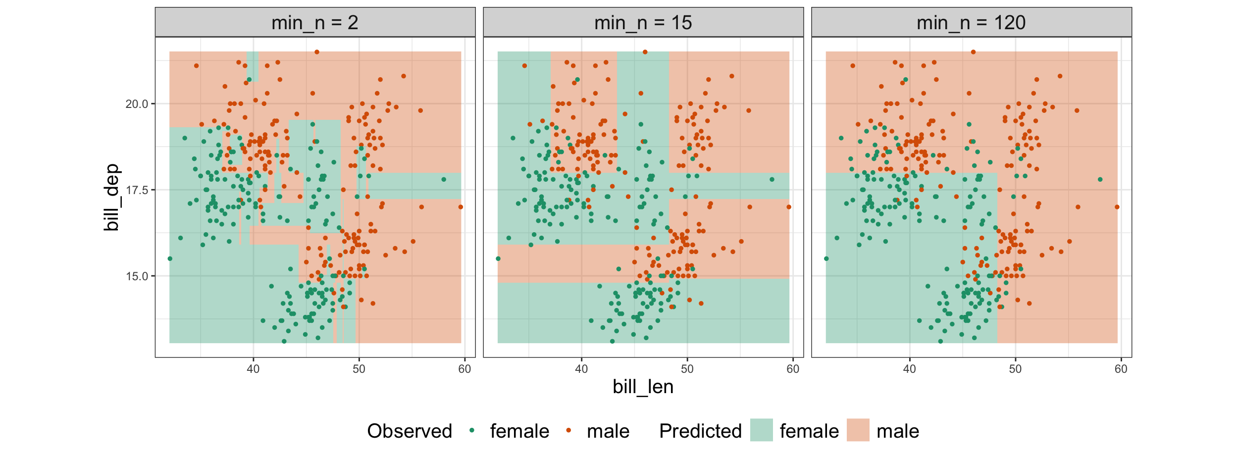
A tree keeps splitting until the regions are pure or too small. The hyperparameter min_n is the minimum number of penguins a region must have to be split again:
Small min_n: many small regions that follow individual penguins: a very flexible tree, like a small \(k\) in KNN
Large min_n: a few big regions: a simple tree
Like \(k\) in KNN, min_n is a hyperparameter, so we can choose it with cross-validation
Here we set cost_complexity = 0, so that min_n alone controls the size of the tree. cost_complexity and tree_depth are two other ways to limit the size of a tree.
Random forest
A bootstrap sample
A bootstrap sample is a new dataset of the same size, drawn from the original data with replacement: pick a row at random, put it back, and repeat.
For example, with 6 penguins:
Original data
1
2
3
4
5
6
Bootstrap sample
2
2
4
5
5
6
Penguins 2 and 5 appear twice; penguins 1 and 3 are left out
Each bootstrap sample is a slightly different version of the data, with no new data needed - A repeated penguin stands in for similar penguins we never measured.
On average, a bootstrap sample contains about 63% of the original rows; the rest are repeats
One tree is unstable
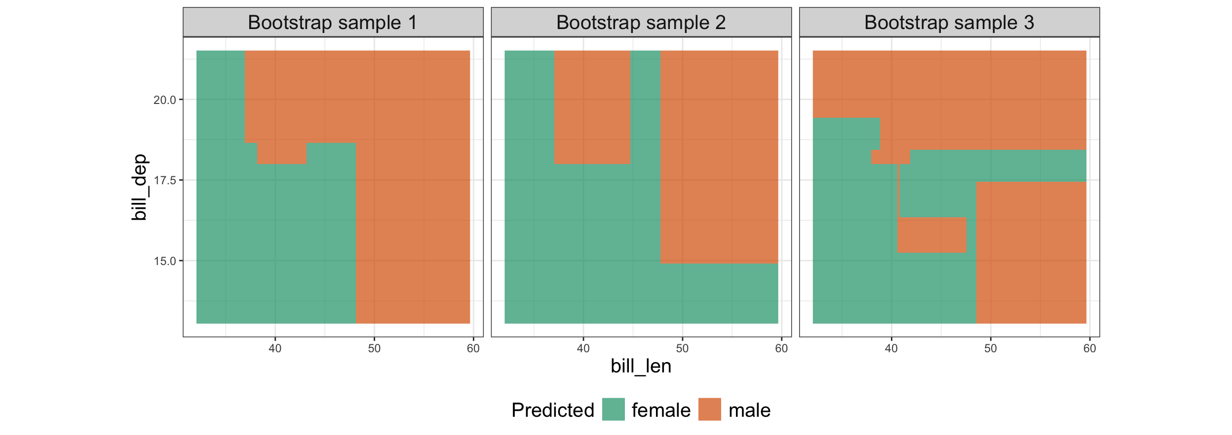
Fit the same classification tree for sex (min_n = 15) on three bootstrap samples of the 333 penguins:
Small changes in the data give very different trees: a single tree has high variance, just like KNN with \(k = 1\).
Lesson from KNN: averaging over many neighbors gave a much more stable prediction. Can we average over many trees?
Grow a forest
A random forest grows many trees (default 500), each one a little different, and lets them vote:
Random rows: each tree is fit on its own bootstrap sample of the training data (as on the previous slide)
Random predictors: at each split, a tree may only choose from a random subset of mtry predictors
Why step 2? If one predictor is very strong, every tree would split on it first, and all the trees would look alike: averaging similar trees doesn’t reduce the variance much. Hiding it from some splits makes the trees different, so their average is more stable.
To predict, combine the trees:
majority vote for classification: rand_forest(mode = "classification") or
the average for regression: rand_forest(mode = "regression").
Combining 500 trees: majority vote
A new penguin with bill_len = 41 and bill_dep = 16: ask every tree in the forest. Tree \(k\) is the tree (min_n = 15) on bootstrap sample \(k\)
Vote
Tree 1
female
Tree 2
female
Tree 3
male
Tree 4
male
Tree 5
female
Tree 6
male
…
…
Tree 500
male
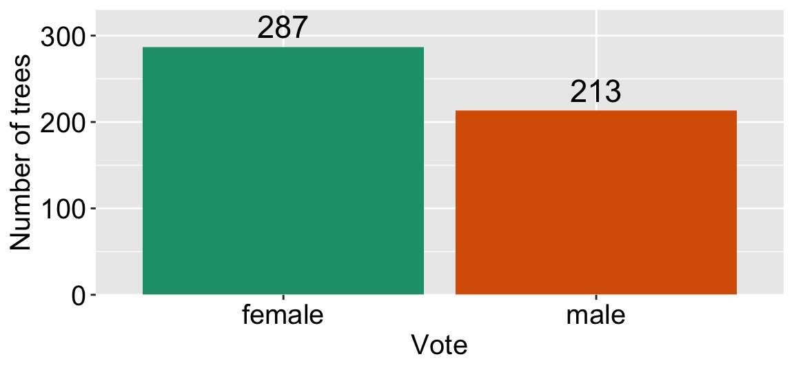
Final prediction: female, the majority: 287 of the 500 trees vote female, even though some trees disagree
From individual trees to the final prediction
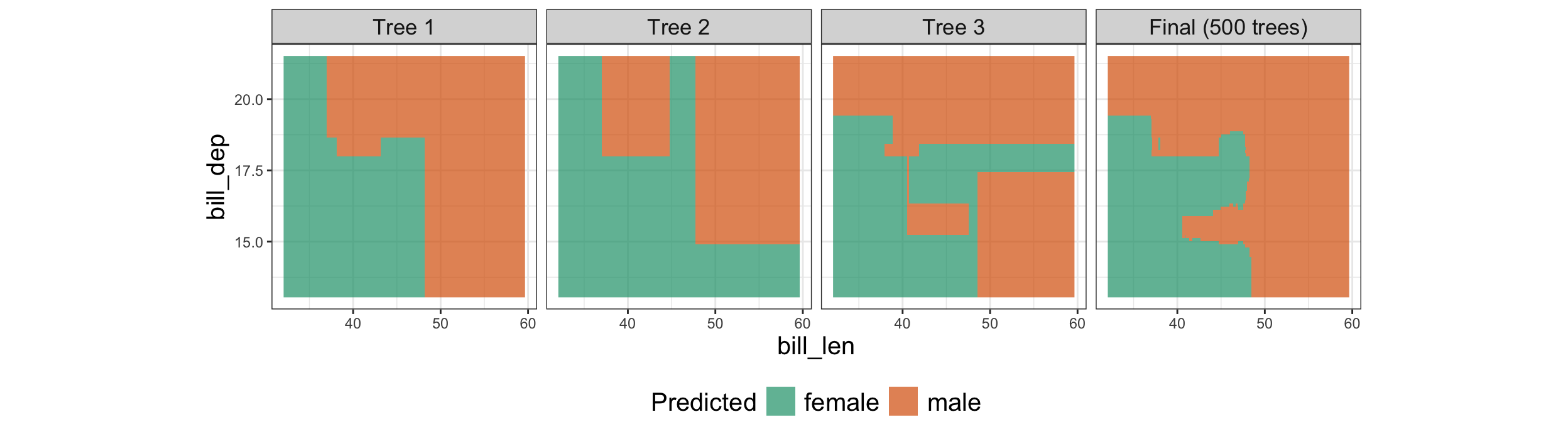
Do this vote at every point of the space: trees 1 to 3 (the same trees as on bootstrap samples 1 to 3), and the final prediction of all 500 trees
Each tree is blocky and makes mistakes in different places: each has its own bootstrap sample
Far from the boundary, almost every tree agrees. Near it, the trees disagree, and the vote settles it
The final prediction is more stable than any single tree: changing a few trees barely changes the vote
Hyperparameters of a random forest
min_n: how deep each tree grows, as in a single tree
small: deep, flexible trees; large: shallow, simple trees
tune it
mtry (new): how many predictors each split can choose from
small: the trees are very different; large: the trees are very similar
tune it
trees (new): how many trees to average
few: unstable predictions; many: stable, but slower to fit
don’t tune it: just use enough (the default, 500)
trees: more trees never hurt
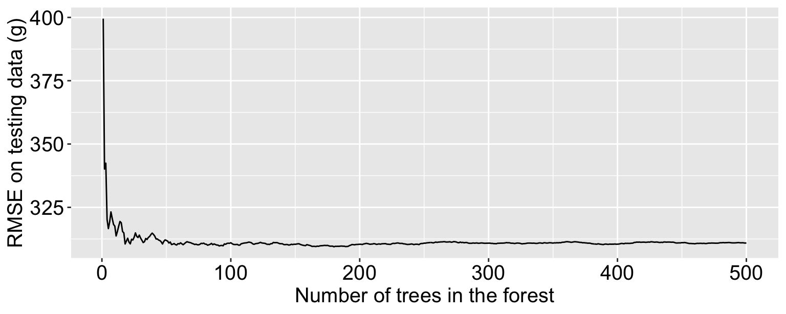
Example (as in the tuning workflow): predict body_mass from the other six penguin variables, and compute the RMSE on the testing data
One tree: RMSE 400 g. Averaging more trees quickly brings it down, and after about 100 trees it stays flat at about 311 g
Adding trees never makes the forest overfit: it only takes longer to fit. So we don’t tune trees, we just use enough of them (the default, 500, is plenty here)
mtry: how different are the trees?
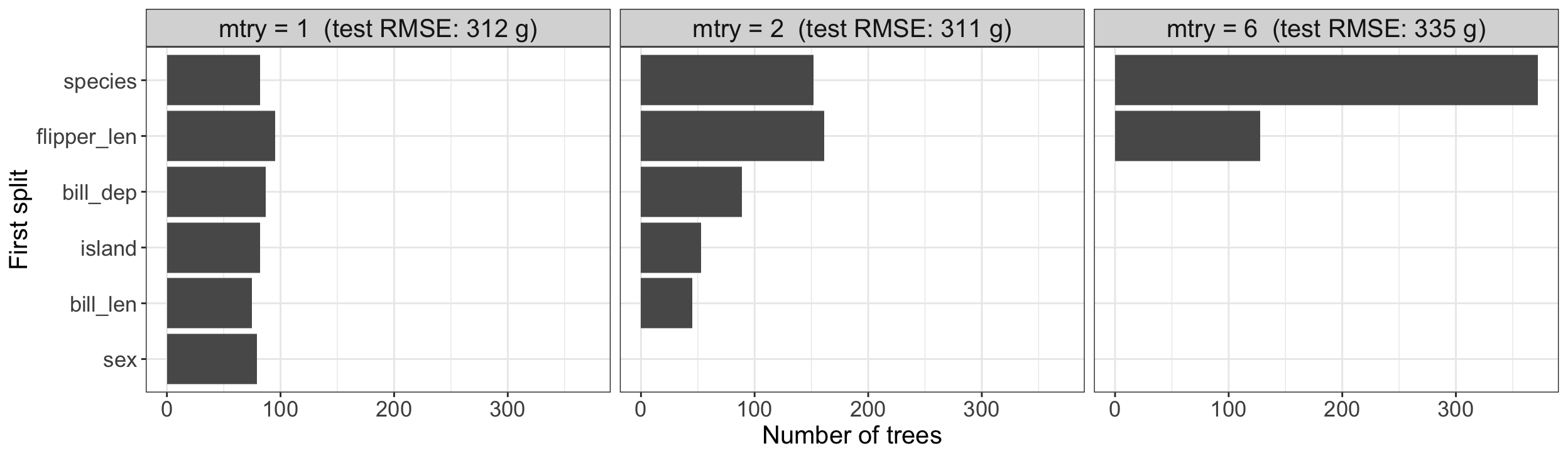
Which predictor does each of the 500 trees split on first?
mtry = 6 (all predictors): every tree picks the strongest predictors (species, flipper_len) first, so the trees are near-copies, and averaging copies doesn’t reduce the variance much
Small mtry: the trees are forced to use different predictors, so they are different, and their average is more stable. But if mtry is too small, each tree is too weak
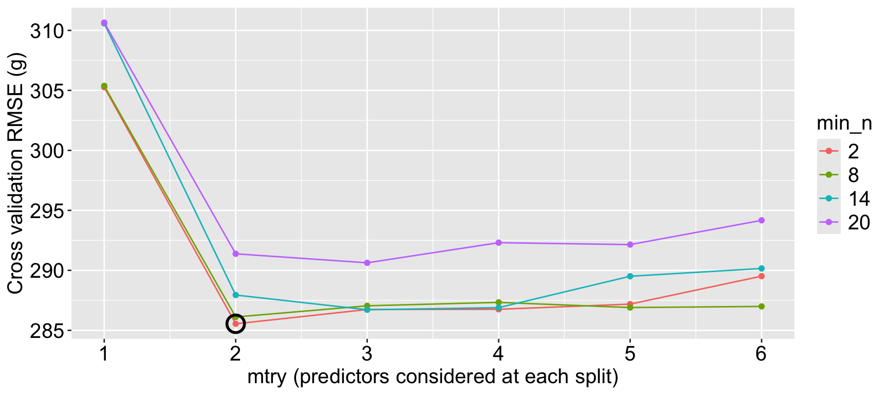
The best mtry is somewhere in between, and depends on the data: tune it with cross-validation
Random forest workflow with tuning and CV
Step 0: Training-testing split
Step 1: Specify the model, with mtry and min_n left to tune
Step 2: Specify the pre-processing recipe
Step 3: Build a workflow
Step 4: Fit the model
4a: Generate the cross validation folds from the training data
4b: Generate the hyperparameter grid
4c: Fit the model on the cv folds and hp grid
4d: Average the metrics over the folds
4e: Find the best model
4f: Plug in the best values and refit on the whole training data
Step 5/6: Predict and calculate prediction accuracy metrics on the testing data
Random forest workflow with tuning and CV
Predict body_mass from the other six penguin variables.
One column per hyperparameter we set to tune(): mtry and min_n
levels = c(6, 4): 6 values of mtry (1 to 6) \(\times\) 4 values of min_n (2, 8, 14, 20) = 24 combinations: every value of mtry is paired with every value of min_n
Random forest workflow with tuning and CV
Step 4c: Fit the forest for every combination on every fold