Elements of Data Science
H. Sherry Zhang
Learning objectives
Training-testing split
rsample initial_split(), training(), testing()
Set up a pre-processing recipe
recipes recipe(), step_*(), all_predictors()
Set up a model
parsnip linear_reg(), logistic_reg(), nearest_neighbor(), set_engine()
Set up a model workflow
workflows workflow(), add_recipe(), add_model()
Fit a model
infer / rsample fit(), vfold_cv(), fit_resamples(), collect_metrics()
Extract the model output
broom glance(), tidy(), augment()
Calculate model metrics
yardstick metrics(), conf_mat(), roc_curve(), autoplot()
Roadmap
Example #1: A basic linear model
Your time: apply the workflow for logistic regression
Example #2: Add the training-testing split for logistic regression
Your time: apply the training-testing split for KNN classification
Example #3: Add cross-validation for KNN classification
Example #4: Add hyper-parameter tuning with cross-validation for KNN classification
Follow along the class example with
usethis::create_from_github(SDS322E-2025Fall/1103-tidymodels")
Example #1 : linear model
Step 1: Specify the model:
<- parsnip:: linear_reg () |> parsnip:: set_engine ("lm" )
Step 2: Specify the pre-processing steps:
<- recipes:: recipe (body_mass ~ flipper_len + bill_len + bill_dep, data = datasets:: penguins) |> :: step_naomit (recipes:: all_predictors ())
Step 3: Build a workflow:
<- workflows:: workflow () |> workflows:: add_recipe (lm_rec) |> workflows:: add_model (lm_mod)
Step 4: Fit the model:
<- lm_wf |> infer:: fit (data = datasets:: penguins)
Step 5: Predict:
<- broom:: augment (lm_fit, datasets:: penguins)
Step 6: Calculate classification metrics:
<- yardstick:: metrics (res_lm, truth = body_mass, estimate = .pred)
Your time
Can you replicate the example to fit a logistic regression?
Step 1: you will be using the lgoistic_reg(), which engine to use?
Step 2: preprocessing
Step 3: build a workflow to combine the model and recipe
Step 4: fit the model
Step 5: obtain the prediction
Step 6: obtain the accuracy metric.
If you have extra time,
read the documentation of the function conf_mat() and obtain the confusion matrix
read the documentation of the function roc_curve() and plot the ROC curve
Solution
Step 1: Specify the model:
<- parsnip:: logistic_reg () |> parsnip:: set_engine ("glm" )
Step 2: Specify the preprocessing step:
<- recipes:: recipe (sex ~ flipper_len + bill_len + bill_dep, data = datasets:: penguins) |> :: step_naomit (recipes:: all_predictors ())
Step 3: Build a workflow:
<- workflows:: workflow () |> workflows:: add_recipe (lr_rec) |> workflows:: add_model (lr_mod)
Step 4: Fit the model:
<- lr_wf |> infer:: fit (data = datasets:: penguins)
Step 5: Predict:
<- broom:: augment (lr_fit, datasets:: penguins) # obtain the prediction on the original dataset
Solution
Step 6: Obtain accuracy measures:
:: conf_mat (res_lr, sex, estimate = .pred_class)
          Truth
Prediction female male
    female    134   32
    male       31  136
:: metrics (res_lr, truth = .pred_class, estimate = sex)
# A tibble: 2 × 3
  .metric  .estimator .estimate
  <chr>    <chr>          <dbl>
1 accuracy binary         0.811
2 kap      binary         0.622
More metrics calculated in the wild:
summary (conf_mat (res_lr, sex, estimate = .pred_class))
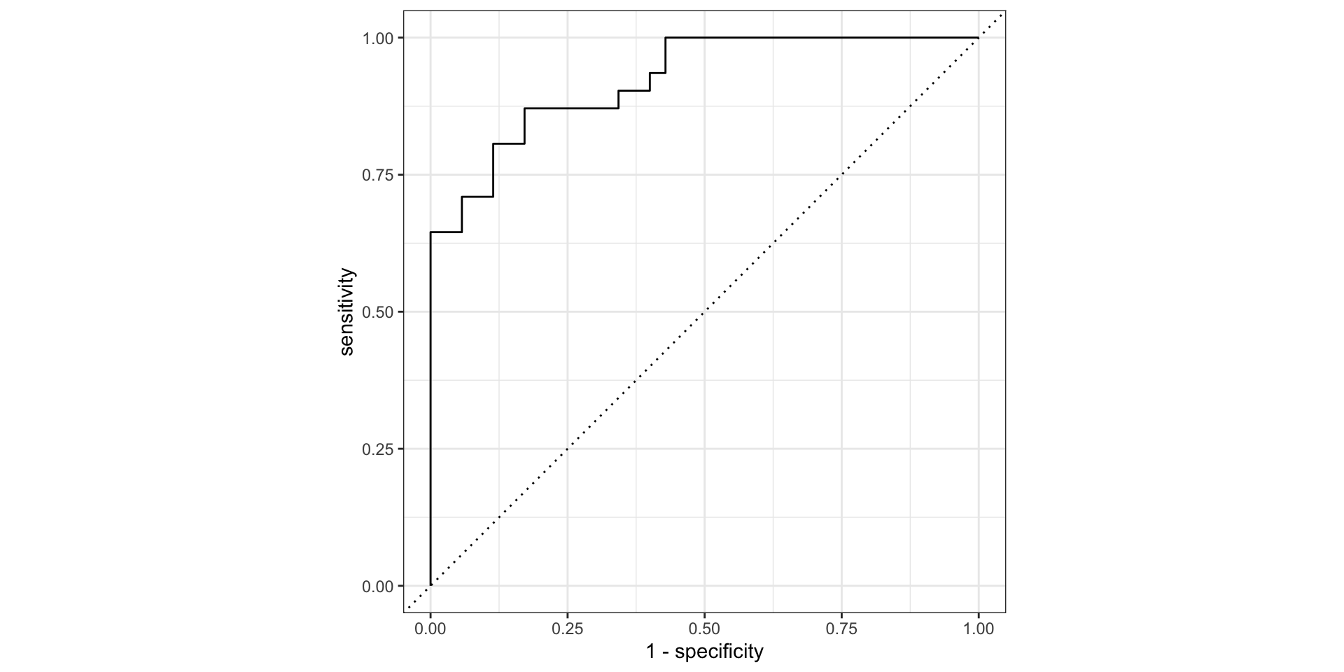
<- yardstick:: roc_curve (res_lr, truth = sex, .pred_female)autoplot (roc_data)
Example #2: Add training-testing split Step 0: Training-testing split: new
set.seed (123 )<- rsample:: initial_split (datasets:: penguins, prop = 0.8 )<- rsample:: training (penguins_split)<- rsample:: testing (penguins_split)
Step 1/2/3: Specify the model/pre-processing recipe/workflow:
<- parsnip:: logistic_reg () %>% parsnip:: set_engine ("glm" )<- recipes:: recipe (sex ~ flipper_len + bill_len + bill_dep, data = penguins_train) |> :: step_naomit (recipes:: all_predictors ())<- workflows:: workflow () |> workflows:: add_recipe (lr_rec) |> workflows:: add_model (lr_mod)
Step 4: Fit the model: train on the training data
<- lr_wf |> infer:: fit (data = penguins_train)
Step 5: Predict: predict on the testing dataset
<- broom:: augment (lr_fit, penguins_test)
Example #2: Add training-testing split Step 6: Calculate classification metrics:
<- yardstick:: conf_mat (res_split, truth = sex, estimate = .pred_class)<- yardstick:: roc_curve (res_split, truth = sex, .pred_female)autoplot (roc_data)
Your time: construct a KNN classification model with training-testing split Step 0: training-testing split
Step 1: Specify the model:
Can you find which model function to use for KNN classification? Which mode? Do you know where to specify the number of neighbors? We will be using the kknn engine
Step 2: Specify the pre-processing recipe:
In KNN, we need to scale the variables (since it is a distance based algorithm) - can you find the correct place to add the scaling step?
Step 3: Construct a workflow to combine the recipe and the model
Step 4: Fit the model on the training data
Step 5: Predict on the testing data
Step 6: Calculate accuracy metrics
Solution
Step 0: training-testing split:
set.seed (123 )<- rsample:: initial_split (datasets:: penguins, prop = 0.8 )<- rsample:: training (penguins_split)<- rsample:: testing (penguins_split)
Step 1: Specify the pre-processing recipe: new
<- recipes:: recipe (sex ~ flipper_len + bill_len + bill_dep, data = penguins_train) |> :: step_naomit (recipes:: all_predictors ()) |> :: step_normalize (recipes:: all_predictors ())
Step 2: Specify the model:
<- parsnip:: nearest_neighbor (mode = "classification" , neighbors = 7 ) |> :: set_engine ("kknn" )
You can also write it as:
nearest_neighbor (neighbors = 7 ) |> set_engine ("kknn" ) |> set_mode ("classification" )
Model parameters, e.g. neighbors = 7, are always specified within the model, nearest_neighbor() - we will look at more complicated cases on how to tune this parameter later.
Solution
Step 3: Build a workflow:
<- workflows:: workflow () |> workflows:: add_recipe (penguins_rec) |> workflows:: add_model (knn_mod)
Step 4: Fit the model:
<- knn_wf |> infer:: fit (data = penguins_train)
Step 5/6: Predict and calculate accuracy metrics:
<- broom:: augment (knn_fit, penguins_test):: metrics (res_knn, truth = sex, estimate = .pred_class)
# A tibble: 2 × 3
  .metric  .estimator .estimate
  <chr>    <chr>          <dbl>
1 accuracy binary         0.864
2 kap      binary         0.724
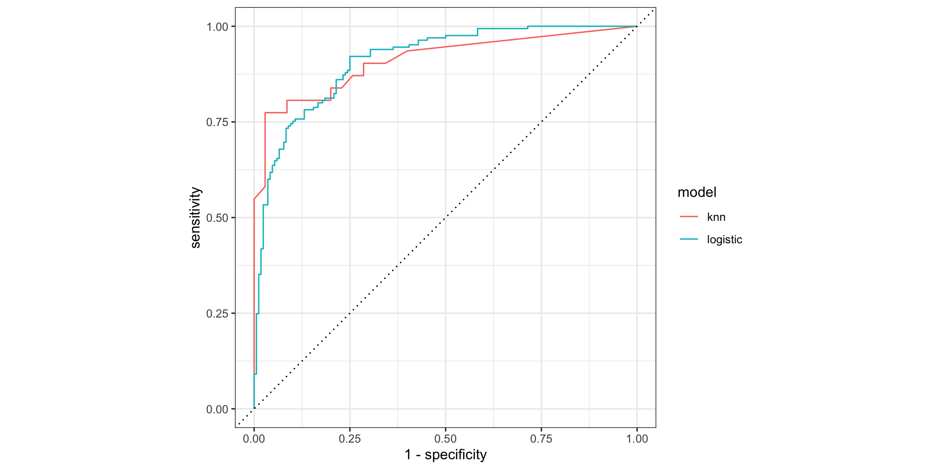
From logistic regression:
:: metrics (res_lr, truth = sex, estimate = .pred_class)
# A tibble: 2 × 3
  .metric  .estimator .estimate
  <chr>    <chr>          <dbl>
1 accuracy binary         0.811
2 kap      binary         0.622
|> mutate (model = "knn" ) |> bind_rows (res_lr |> mutate (model = "logistic" )) |> group_by (model) |> roc_curve (sex, .pred_female) |> autoplot ()
Example: Cross validation with KNN
Step 1: Specify the model
Step 2: Specify the pre-processing recipe
Step 3: Build a workflow
Step 4: Fit the model
Step 5/6: Predict and calculate classification metrics
Example #3: Cross validation with KNN Step 1/2/3: Specify the pre-processing recipe, the model, and the workflow - same
<- datasets:: penguins |> na.omit ()set.seed (123 )<- rsample:: initial_split (penguins_clean, prop = 0.8 )<- rsample:: training (penguins_split)<- rsample:: testing (penguins_split)<- recipe (sex ~ bill_len + bill_dep + flipper_len, data = penguins_train) |> step_normalize (all_predictors ())<- nearest_neighbor (mode = "classification" , neighbors = 7 ) |> set_engine ("kknn" )<- workflow () |> add_recipe (penguins_rec) |> add_model (knn_mod)
Step 4: Generate the cross validation sampling/ Fit the model
<- rsample:: vfold_cv (penguins_train, v = 10 )<- fit_resamples (wf, resamples = penguins_folds)|> collect_metrics ()
# A tibble: 3 × 6
  .metric     .estimator   mean     n std_err .config
  <chr>       <chr>       <dbl> <int>   <dbl> <chr>
1 accuracy    binary     0.865     10 0.0151  Preprocessor1_Model1
2 brier_class binary     0.0987    10 0.00930 Preprocessor1_Model1
3 roc_auc     binary     0.936     10 0.0128  Preprocessor1_Model1
Example #3: Cross validation with KNN
<- fit_resamples (wf, resamples = penguins_folds)$ .metrics[[1 ]]
# A tibble: 3 × 4
  .metric     .estimator .estimate .config
  <chr>       <chr>          <dbl> <chr>
1 accuracy    binary         0.778 Preprocessor1_Model1
2 roc_auc     binary         0.868 Preprocessor1_Model1
3 brier_class binary         0.138 Preprocessor1_Model1
The accuracy metrics here is the average of the 10 folds:
|> collect_metrics ()
# A tibble: 3 × 6
  .metric     .estimator   mean     n std_err .config
  <chr>       <chr>       <dbl> <int>   <dbl> <chr>
1 accuracy    binary     0.865     10 0.0151  Preprocessor1_Model1
2 brier_class binary     0.0987    10 0.00930 Preprocessor1_Model1
3 roc_auc     binary     0.936     10 0.0128  Preprocessor1_Model1
Step 5: Predict
fit (wf, data = penguins_train) |> augment (penguins_test)
Example #4: hyper-parameter tuning with CV Cross validation is more useful for hyper-parameter tuning - e.g. choosing the best number of neighbors in KNN.
Step 1: Specify the model
Step 2: Specify the pre-processing recipe
Step 3: Build a workflow
Step 4: Fit the model
Generate the cross validation sampling Generate the hyperparameter grid Fit the model on the cv folds and hp grid Find the best model Step 5/6: Predict and calculate classification metrics
Example #4: hyper-parameter tuning with CV Step 1/2/3: Specify the pre-processing recipe, the model, and the workflow - same
<- datasets:: penguins |> na.omit ()set.seed (123 )<- initial_split (penguins_clean, prop = 0.8 )<- training (penguins_split)<- testing (penguins_split)<- recipe (sex ~ bill_len + bill_dep, data = penguins_train) |> step_normalize (all_predictors ()) <- nearest_neighbor (mode = "classification" , neighbors = tune:: tune ()) |> set_engine ("kknn" )<- workflow () |> add_recipe (penguins_rec) |> add_model (knn_spec)
Step 4: Generate the cross validation sampling
<- vfold_cv (penguins_train, v = 10 )<- dials:: grid_regular (dials:: neighbors (range = c (1 , 20 )), levels = 20 )# rather than using `fit_resamples()` we use `tune_grid()` <- tune:: tune_grid (knn_wf, resamples = penguins_folds, grid = knn_grid)head (knn_res, 3 )
# A tibble: 3 × 4
  splits           id     .metrics          .notes
  <list>           <chr>  <list>            <list>
1 <split [239/27]> Fold01 <tibble [60 × 5]> <tibble [1 × 3]>
2 <split [239/27]> Fold02 <tibble [60 × 5]> <tibble [1 × 3]>
3 <split [239/27]> Fold03 <tibble [60 × 5]> <tibble [1 × 3]>
Example #4: hyper-parameter tuning with CV
# look at accuracy for all the models: knn_res |> collect_metrics() <- knn_res |> select_best (metric = "roc_auc" )
# A tibble: 1 × 2
  neighbors .config
      <int> <chr>
1        20 Preprocessor1_Model20
<- finalize_workflow (knn_wf, best_k)
Step 5: Predict
finalize_workflow (knn_wf, best_k) |> fit (data = penguins_train) |> augment (penguins_test)