Linear Regression Model Specification (regression)

Computational engine: lm Elements of Data Science
SDS 322E
H. Sherry Zhang
Department of Statistics and Data Sciences
University of Texas at Austin
Get the repository for today:
library(usethis) create_from_github("SDS322E-26FALL/1002-tidymodels", fork = FALSE)
Learning objectives
Understand the six-step tidymodels workflow: specify the model, specify the pre-processing, combine them, fit, predict, and evaluate
Apply the workflow to a linear regression (example: penguin
body_mass)Apply the same workflow to a logistic regression (your turn: penguin
sex)
Follow along the class example with
usethis::create_from_github("SDS322E-26FALL/1002-tidymodels")
The same six steps work for almost every model: switching from linear to logistic regression (or KNN, random forest, …) only changes the model specification.
In later lectures when we cover KNN and random forest, we will also cover training-testing split and cross-validation (rsample), and hyper-parameter tuning (tune).
The tidymodels toolkit
| Step | What you do | Package | Key functions |
|---|---|---|---|
| 1 | Specify the model | parsnip | linear_reg(), logistic_reg(), set_engine() |
| 2 | Specify the pre-processing | recipes | recipe(), step_*(), all_predictors() |
| 3 | Combine model + recipe | workflows | workflow(), add_model(), add_recipe() |
| 4 | Fit the model | workflows | fit() |
| 5 | Predict and inspect the output | broom | augment(), tidy(), glance() |
| 6 | Evaluate the model | yardstick | metrics(), conf_mat(), roc_curve(), autoplot() |
Example: linear regression
Step 1: specify the model - parsnip
Goal: predict penguin body_mass from flipper_len, bill_len, and bill_dep with a linear regression.
First, tell tidymodels what kind of model to fit (linear_reg()) and which engine to use to fit it (set_engine("lm"), i.e. the lm() function we already know):
This is only a specification: no data is involved yet and nothing has been fitted.
Step 2: pre-processing - recipes
A recipe records the formula (outcome ~ predictors) and the data preparation steps:
── Recipe ────────────────────────────

── Inputs
Number of variables by role
outcome:   1
predictor: 3

── Operations
• Removing rows with NA values in: recipes::all_predictors()datahere is only used to learn the variable names and typesstep_naomit()removes rows with missing values;all_predictors()selects all the predictor variables- Other
step_*()functions:step_normalize(),step_dummy(),step_log(), …
Step 3: build a workflow - workflows
A workflow bundles the model (step 1) and the recipe (step 2) together:
lm_wf <- workflows::workflow() |> workflows::add_recipe(lm_rec) |> workflows::add_model(lm_mod)
lm_wf
══ Workflow ════════════════════════════════════════════════════════════════════
Preprocessor: Recipe
Model: linear_reg()
── Preprocessor ────────────────────────────────────────────────────────────────
1 Recipe Step
• step_naomit()
── Model ───────────────────────────────────────────────────────────────────────
Linear Regression Model Specification (regression)
Computational engine: lm Still nothing has been fitted, but the workflow now has everything it needs.
Step 4: fit the model - infer
Now we give the workflow the data:
══ Workflow [trained] ══════════════════════════════════════════════════════════
Preprocessor: Recipe
Model: linear_reg()

── Preprocessor ────────────────────────────────────────────────────────────────
1 Recipe Step

• step_naomit()

── Model ───────────────────────────────────────────────────────────────────────

Call:
stats::lm(formula = ..y ~ ., data = data)

Coefficients:
(Intercept)  flipper_len     bill_len     bill_dep
  -6424.765       50.269        4.162       20.050
These are the same coefficients you would get from lm(body_mass ~ flipper_len + bill_len + bill_dep, data = penguins).
Step 5: predict - broom
broom::augment() adds the predictions (.pred) and residuals (.resid) as new columns to the data:
res_lm <- broom::augment(lm_fit, datasets::penguins)
res_lm |> select(.pred, .resid, body_mass, flipper_len, bill_len, bill_dep)
# A tibble: 344 × 6
.pred .resid body_mass flipper_len bill_len bill_dep
<dbl> <dbl> <int> <int> <dbl> <dbl>
1 3212. 538. 3750 181 39.1 18.7
2 3439. 361. 3800 186 39.5 17.4
3 3906. -656. 3250 195 40.3 18
4 NA NA NA NA NA NA
5 3817. -367. 3450 193 36.7 19.3
6 3703. -53.0 3650 190 39.3 20.6
7 3193. 432. 3625 181 38.9 17.8
8 3934. 741. 4675 195 39.2 19.6
9 3782. -307. 3475 193 34.1 18.1
10 3706. 544. 4250 190 42 20.2
# ℹ 334 more rowsStep 6: evaluate - yardstick
yardstick::metrics() compares the true values (truth) with the predictions (estimate):
# A tibble: 3 × 3
  .metric .estimator .estimate
  <chr>   <chr>          <dbl>
1 rmse    standard     391.
2 rsq     standard       0.761
3 mae     standard     310.
For a regression model, the default metrics are:
rmse: root mean squared errorrsq: R-squaredmae: mean absolute error
Putting it all together
# step 1: specify the model
lm_mod <- parsnip::linear_reg() |> parsnip::set_engine("lm")

# step 2: specify the pre-processing
lm_rec <- recipes::recipe(body_mass ~ flipper_len + bill_len + bill_dep, data = datasets::penguins) |>
  recipes::step_naomit(recipes::all_predictors())

# step 3: combine them in a workflow
lm_wf <- workflows::workflow() |> workflows::add_recipe(lm_rec) |> workflows::add_model(lm_mod)

# step 4: fit the model
lm_fit <- lm_wf |> infer::fit(data = datasets::penguins)

# step 5: predict
res_lm <- broom::augment(lm_fit, datasets::penguins)

# step 6: evaluate the model
res <- yardstick::metrics(res_lm, truth = body_mass, estimate = .pred)
Why do we need data in both step 2 and step 4?
- step 2:
dataonly tells the recipe what the variables look like (names and types) - step 4:
datais what the recipe and the model learn from (won’t be the full data when we do cross-validation or train-test split)
Your time
Can you replicate the example to fit a logistic regression?
- Step 1: you will be using the
logistic_reg(), which engine to use?
- Step 2: preprocessing
- Step 3: build a workflow to combine the model and recipe
- Step 4: fit the model
- Step 5: obtain the prediction
- Step 6: obtain the accuracy metric.
If you have extra time,
- read the documentation of the function
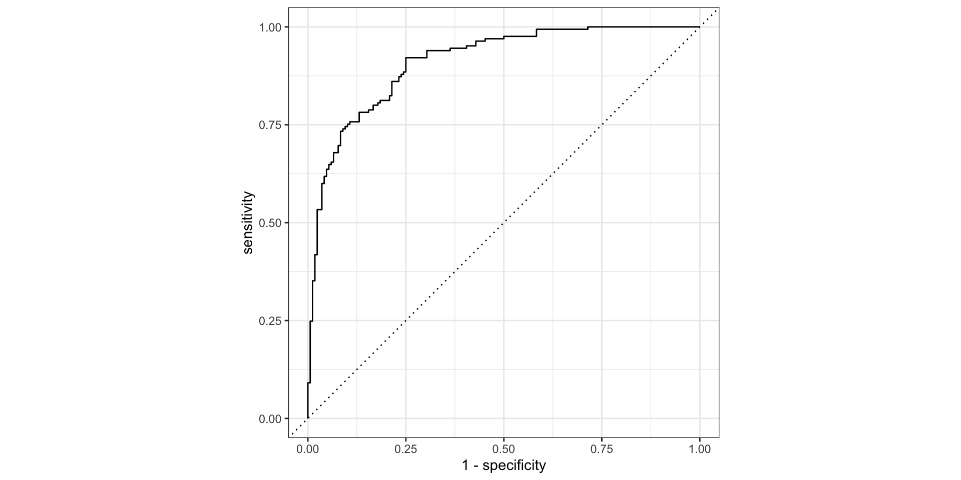
conf_mat()and obtain the confusion matrix - read the documentation of the function
roc_curve()and plot the ROC curve
Solution
Step 1: Specify the model:
Step 2: Specify the preprocessing step:
Step 3: Build a workflow:
Step 4: Fit the model:
Step 5: Predict:
Solution
Step 6: Obtain accuracy measures:
More metrics calculated in the wild: