Elements of Data Science
SDS 322E

H. Sherry Zhang
Department of Statistics and Data Sciences
The University of Texas at Austin

Fall 2025

Learning objectives

  • Understand what problem dimension reduction methods are solving

  • Apply Principal component analysis to the data

    • preprocessing
    • compute pca with prcomp()
    • extract the first x PCs: broom::augment()
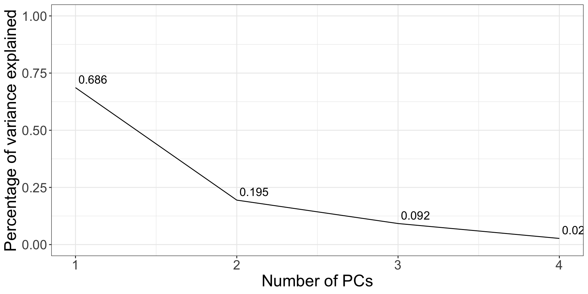
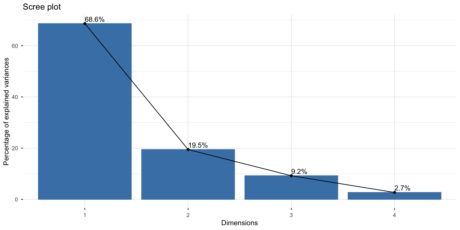
    • observe the screen plot to find the optimal number of PCs
    • plot the data projected onto the first two PCs

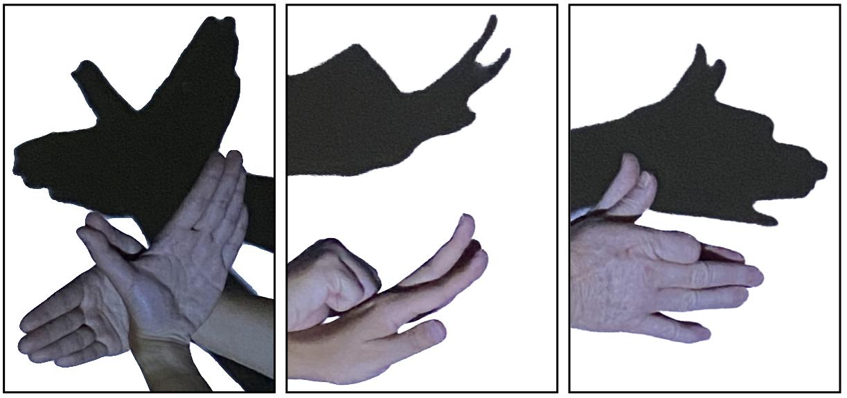
Motivation - dimension reduction

  • Hand shadow puppet: 3D hand poses reduced to 2D shadows (Projection)

We want the projection to resemble the original data as much as possible.

Principal component analysis

  • Principal component analysis is a linear dimension reduction technique that finds a low-dimensional representation of a dataset that contains as much as possible of the variation.
  • It can be formulated as an optimization problem to maximize the variance of the projected data, subject to some constraint.

  • The solution to the optimization happens to be the singular value decomposition of the data matrix \(X\) (if the data has column mean of zero).

  • All of these will be taken care of by the function prcomp().

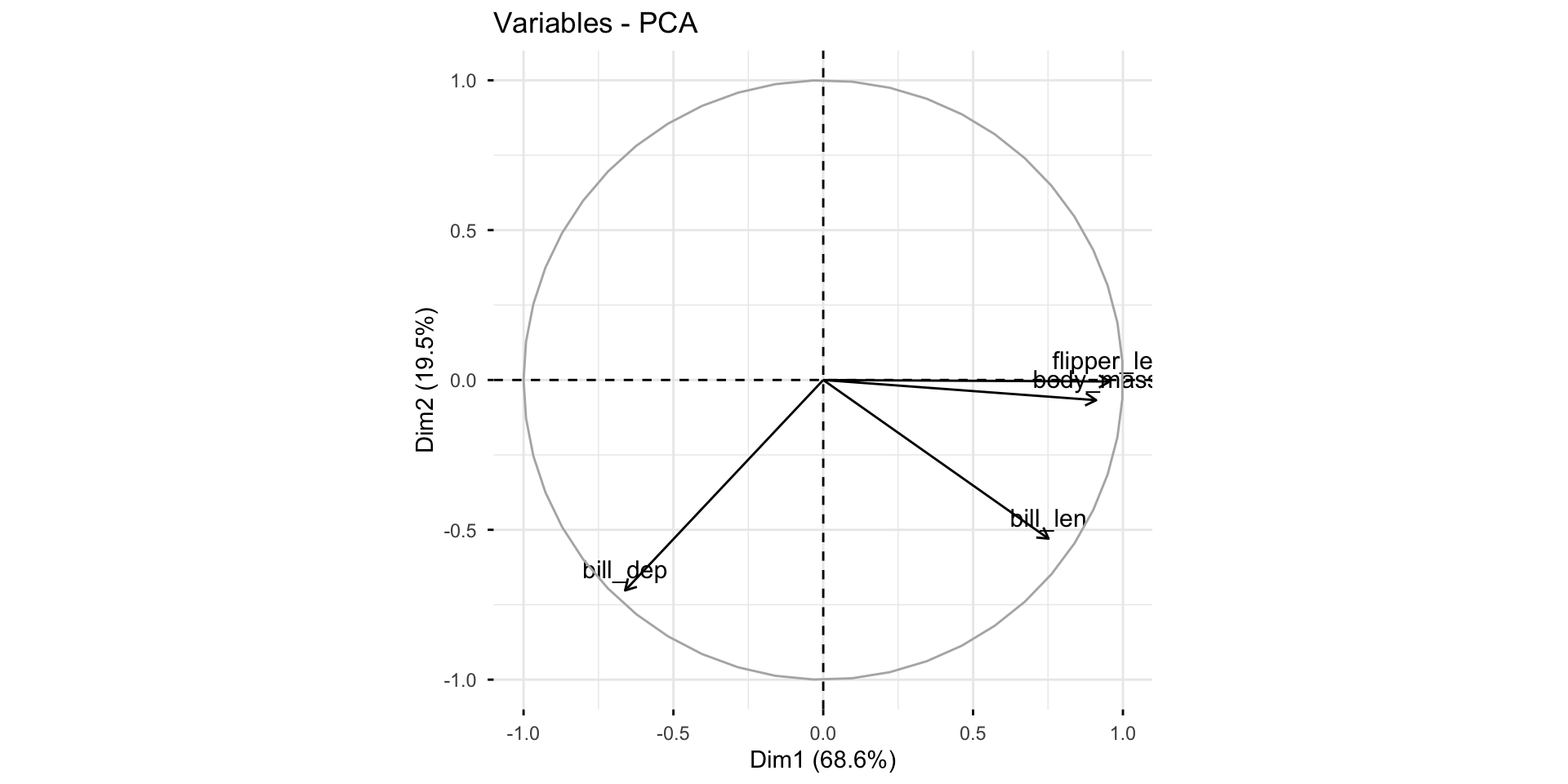
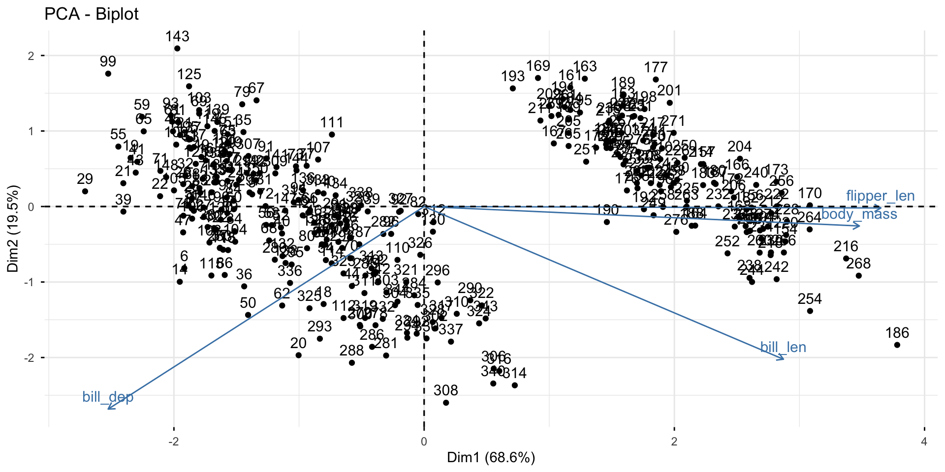
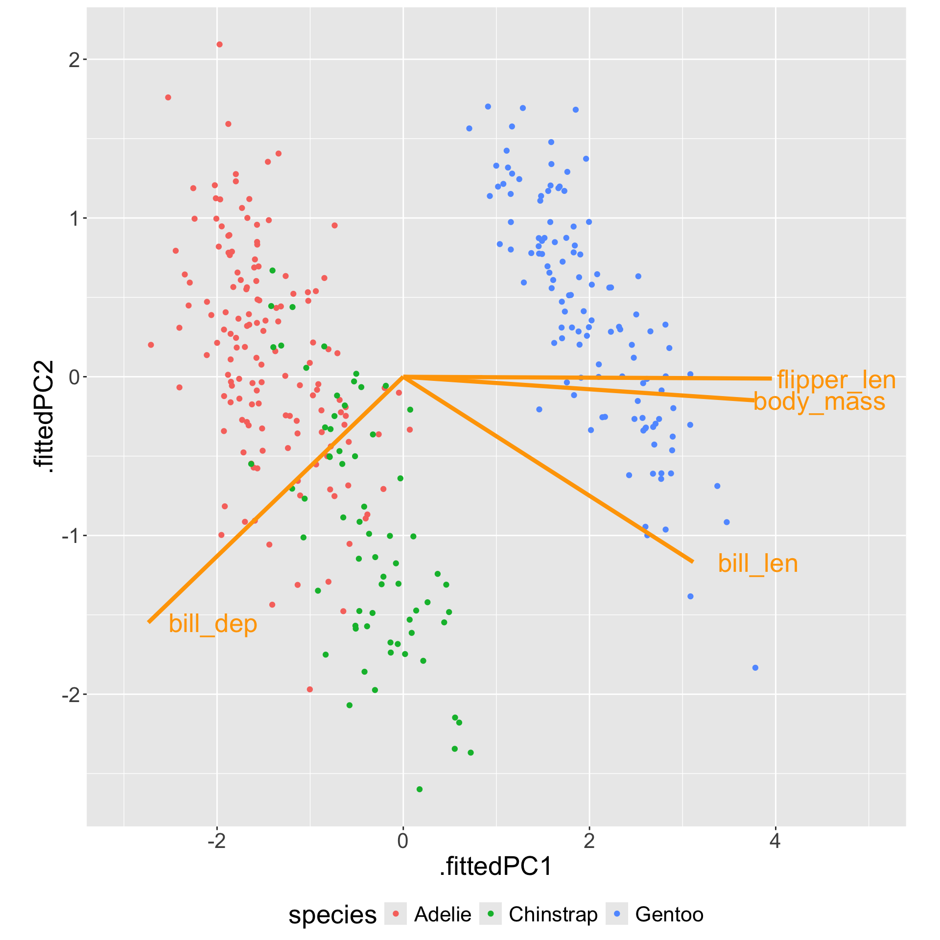
PCA example - Penguins data again

library(tidyverse)
as_tibble(penguins)
# A tibble: 344 × 8
  species island    bill_len bill_dep flipper_len body_mass sex     year
  <fct>   <fct>        <dbl>    <dbl>       <int>     <int> <fct>  <int>
1 Adelie  Torgersen     39.1     18.7         181      3750 male    2007
2 Adelie  Torgersen     39.5     17.4         186      3800 female  2007
3 Adelie  Torgersen     40.3     18           195      3250 female  2007
4 Adelie  Torgersen     NA       NA            NA        NA <NA>    2007
5 Adelie  Torgersen     36.7     19.3         193      3450 female  2007
# ℹ 339 more rows

Would you think missing values would be a problem for PCA?

penguins_clean <- penguins |> na.omit()
penguins_clean |> head()
  species    island bill_len bill_dep flipper_len body_mass    sex year
1  Adelie Torgersen     39.1     18.7         181      3750   male 2007
2  Adelie Torgersen     39.5     17.4         186      3800 female 2007
3  Adelie Torgersen     40.3     18.0         195      3250 female 2007
5  Adelie Torgersen     36.7     19.3         193      3450 female 2007
6  Adelie Torgersen     39.3     20.6         190      3650   male 2007
7  Adelie Torgersen     38.9     17.8         181      3625 female 2007

PCA example - Penguins data

The function prcomp() in R can be used to perform PCA. The data is centered by default (center = TRUE).

  • We would also like to scale the data (scale = TRUE) since the features are measured in different units (mm vs g).
  • You may separately center and scale the data before applying PCA and set center = FALSE and scale = FALSE.
res_pca <-  prcomp(penguins_clean[, 3:6], scale = TRUE)
res_pca
Standard deviations (1, .., p=4):
[1] 1.6569115 0.8821095 0.6071594 0.3284579

Rotation (n x k) = (4 x 4):
                   PC1         PC2        PC3        PC4
bill_len     0.4537532 -0.60019490 -0.6424951  0.1451695
bill_dep    -0.3990472 -0.79616951  0.4258004 -0.1599044
flipper_len  0.5768250 -0.00578817  0.2360952 -0.7819837
body_mass    0.5496747 -0.07646366  0.5917374  0.5846861

Penguins data - Inspect the PCA results

  • eigenvalue: standard deviations of the principal components - their square capture the variance explained by each PC
res_pca$sdev
[1] 1.6569115 0.8821095 0.6071594 0.3284579
  • rotation: principal components (eigenvectors) - directions of maximum variance
res_pca$rotation
                   PC1         PC2        PC3        PC4
bill_len     0.4537532 -0.60019490 -0.6424951  0.1451695
bill_dep    -0.3990472 -0.79616951  0.4258004 -0.1599044
flipper_len  0.5768250 -0.00578817  0.2360952 -0.7819837
body_mass    0.5496747 -0.07646366  0.5917374  0.5846861
  • center/ scale: column mean and standard deviation (if applicable)
res_pca$center
   bill_len    bill_dep flipper_len   body_mass 
   43.99279    17.16486   200.96697  4207.05706 
res_pca$scale
   bill_len    bill_dep flipper_len   body_mass 
   5.468668    1.969235   14.015765  805.215802 

Diagnostics: Choose k

res_pca_var <- tibble(
  n = 1:length(res_pca$sdev), 
  sd = res_pca$sdev, 
  var = res_pca$sdev^2,
  prop = var/ sum(var))
res_pca_var
# A tibble: 4 × 4
      n    sd   var   prop
  <int> <dbl> <dbl>  <dbl>
1     1 1.66  2.75  0.686 
2     2 0.882 0.778 0.195 
3     3 0.607 0.369 0.0922
4     4 0.328 0.108 0.0270
res_pca_var |> 
  mutate(cum_prop = cumsum(prop))
# A tibble: 4 × 5
      n    sd   var   prop cum_prop
  <int> <dbl> <dbl>  <dbl>    <dbl>
1     1 1.66  2.75  0.686     0.686
2     2 0.882 0.778 0.195     0.881
3     3 0.607 0.369 0.0922    0.973
4     4 0.328 0.108 0.0270    1    
ggplot(res_pca_var, aes(x = n, y = prop)) + 
  geom_line() +
  geom_text(aes(label = round(prop, 3)), 
            vjust = -0.5, hjust = -0.1,
            size = 5) +
  xlab("Number of PCs") + 
  ylab("Percentage of variance explained") +
  theme_bw() + 
  theme(text = element_text(size = 20)) + 
  ylim(0, 1)

This plot is called a scree plot - used to tell the number of principal components to retain. Choose the number at the “elbow” point: k = 2 here.

Scree plot

The fviz_screeplot() function from the factoextra package allows you to plot the scree plot in one command.

factoextra::fviz_eig(res_pca, addlabels = TRUE)

Diagnostics: plot the first 2 PCs

Obtain the projected data:

Option 1: use base R predict()

as_tibble(predict(res_pca))
# A tibble: 333 × 4
    PC1     PC2     PC3    PC4
  <dbl>   <dbl>   <dbl>  <dbl>
1 -1.85 -0.0320  0.235   0.528
2 -1.31  0.443   0.0274  0.401
3 -1.37  0.161  -0.189  -0.528
4 -1.88  0.0123  0.628  -0.472
5 -1.92 -0.816   0.700  -0.196
# ℹ 328 more rows

Option 2: use broom::augment()

fitted_df <- res_pca |> broom::augment(penguins_clean)
fitted_df
# A tibble: 333 × 13
  .rownames species island    bill_len bill_dep flipper_len body_mass
  <chr>     <fct>   <fct>        <dbl>    <dbl>       <int>     <int>
1 1         Adelie  Torgersen     39.1     18.7         181      3750
2 2         Adelie  Torgersen     39.5     17.4         186      3800
3 3         Adelie  Torgersen     40.3     18           195      3250
4 5         Adelie  Torgersen     36.7     19.3         193      3450
5 6         Adelie  Torgersen     39.3     20.6         190      3650
# ℹ 328 more rows
# ℹ 6 more variables: sex <fct>, year <int>, .fittedPC1 <dbl>,
#   .fittedPC2 <dbl>, .fittedPC3 <dbl>, .fittedPC4 <dbl>

Diagnostics: plot the first 2 PCs

factoextra::fviz_pca_var(res_pca)

Diagnostics: plot the first 2 PCs

factoextra::fviz_pca_biplot(res_pca)

Diagnostics: plot the first 2 PCs

  • Gentoo can be separated from the other two species by bill depth (PC1).

  • Among Adelie and Chinstrap, bill length helps separate them (PC2).

This matches with the summary statistics:

# A tibble: 3 × 3
  species   bill_dep bill_len
  <fct>        <dbl>    <dbl>
1 Adelie        18.3     38.8
2 Chinstrap     18.4     48.8
3 Gentoo        15.0     47.6

What’s more

  • Principal component analysis (PCA) is a linear dimension reduction method, there are other linear methods, e.g.
    • Projection Pursuit (PP)
  • There are also non-linear dimension reduction methods, e.g. 
    • Multidimensional Scaling (MDS),
    • T-stochastic Neighbourhood Embedding (t-SNE), and
    • Uniform manifold Approximation and Projection (UMAP)

Appendix

Data:

\[\begin{aligned} X_{n\times p} & = [X_{1} \enspace X_{2} \enspace \dots \enspace X_{p}]_{n\times p} \\ & = \left[ \begin{array}{cccc} x_{11} & x_{12} & \dots & x_{1p} \\ x_{21} & x_{22} & \dots & x_{2p}\\ \vdots & \vdots & & \vdots \\ x_{n1} & x_{n2} & \dots & x_{np} \end{array} \right]_{n\times p} \end{aligned}\]

We require column means of \(X\) to be zero (centered data): \(\bar{X_i} = 0\)

Projected data: \[\begin{aligned} Z_{n\times k} = X\Phi &=[Z_{1} \enspace \dots \enspace Z_{k}]_{n\times k} \\ & = \left[ \begin{array}{cccc} z_{11} & \dots & z_{1k} \\ z_{21} & \dots & z_{2k}\\ \vdots & & \vdots \\ z_{n1} & \dots & z_{nk} \end{array} \right]_{n\times k} \end{aligned}\]

Principal component analysis

In PCA, \(\Phi\) is called the rotation or the loading matrix:

\[\begin{aligned} \Phi_{p \times k} & = [\phi_{1} \enspace \phi_{2} \enspace \dots \enspace \phi_{k}]_{p\times k} \\ & = \left[ \begin{array}{cccc} \phi_{11} & \phi_{12} & \dots & \phi_{1k} \\ \phi_{21} & \phi_{22} & \dots & \phi_{2k}\\ \vdots & \vdots & & \vdots \\ \phi_{p1} & \phi_{p2} & \dots & \phi _{pk} \end{array} \right]_{p\times k} \end{aligned}\]

\(\Phi\) satisfies two conditions:

  • It is normalized: \(\sum _{i=1}^{p} \phi_{ij}^2 = 1\) for \(j = 1, \dots, k\) and
  • Vectors are orthogonal to each other: \(\sum_{i=1}^{p} \phi_{ij}\phi_{ik} = 0\) for \(j \neq k\).

(We will talk about why this is the case in a second.)

Principal component analysis

Principal components are the linear combinations of the original variables:

The first principal component (PC1):

\[\begin{aligned} Z_1 = \begin{bmatrix} z_{11} \\ z_{21} \\ \vdots \\ z_{n1}\end{bmatrix} &= \phi_{11} \begin{bmatrix} x_{11} \\ x_{21} \\ \vdots \\ x_{n1}\end{bmatrix} + \phi_{21} \begin{bmatrix} x_{12} \\ x_{22} \\ \vdots \\ x_{n2}\end{bmatrix} + \dots + \phi_{p1}\begin{bmatrix} x_{1p} \\ x_{2p} \\ \vdots \\ x_{np}\end{bmatrix} \\ &= \phi_{11}X_1 + \phi_{21}X_2 + \dots + \phi_{p1}X_p \\ \end{aligned}\]

where \(\sum _{i=1}^{p} \phi_{i1}^2 = 1\) and \(\bar{Z_i} = 0\) (since \(\bar{X_i} = 0\))

Principal component analysis

For each element in \(Z_1\): \(z_{i1} = \phi_{11}x_{i1} + \phi_{21}x_{i2} + \dots + \phi_{p1}x_{ip} = \sum_{j = 1}^p \phi_{j1} x_{ij}\)

Write down the variance of \(Z_1\):

\[\text{Var}(Z_1) = E(Z_1^2) = \frac{1}{n}\sum_{i = 1}^n z_{i1}^2=\frac{1}{n}\sum_{i = 1}^n (\sum_{j = 1}^p \phi_{j1} x_{ij})^2 \]

We would like to find the direction (the coefficients \(\phi_{j1}\)’s) that maximizes the variance of \(Z_1\):

\[\max_{\phi_{11}, \dots, \phi_{p1}} \text{Var}(Z_1) = \max_{\phi_{11}, \dots, \phi_{p1}} \frac{1}{n}\sum_{i = 1}^n (\sum_{j = 1}^p \phi_{j1} x_{ij})^2 \] subject to the normalization constraint \(\sum _{i=1}^{p} \phi_{i1}^2 = 1\).

Optimization

\[\text{Var}(Z_1) = E(Z_1^2) = \frac{1}{n}\sum_{i = 1}^n z_{i1}^2 = \left\lVert z_{1} \right\rVert^2 = \left\lVert X\phi_1 \right\rVert^2 = \phi_1^T X^T X \phi_1\]

subject to \(\phi_1^T \phi_1 = 1\)

Use Lagrange multipliers to solve the constrained optimization problem:

\[ L(\phi_1, \lambda) = \phi_1^T X^T X \phi_1 - \lambda (\phi_1^T \phi_1 - 1)\] Take the derivative and set it to zero gives \[X^TX\phi_1 = \lambda \phi_1\]

This is the eigenvalue equation for the matrix \(X^TX\).

Recognize \(X^TX\) is related the covariance matrix: \(S = \frac{1}{n-1}X^TX\), the first principal component (\(\phi_1\)) is the eigenvector of \(X^TX\) corresponding to the largest eigenvalue.

Computation

The first principal component (\(\phi_1\)) is the eigenvector of \(X^TX\) corresponding to the largest eigenvalue. This can be obtained through:

  1. Singular value decomposition (SVD) of \(X\) (always apply):

\[X = UDV^T\]

  1. Eigen-decomposition of \(X^TX = (n-1) S\) (since \(X^TX\) is square):

\[X^TX = V D^2 V^T\]

where

  • \(X\) is a \(n \times p\) matrix
  • \(U\) is a \(n \times n\) orthogonal matrix (\(U^TU = 1\))
  • \(D\) is a \(n \times p\) diagonal matrix with non-negative elements (square root of the eigenvalues of \(X^TX\) arranged in descending order)
  • \(V\) is a \(p \times p\) orthogonal matrix (eigenvectors: \(V^TV = 1\))

Principal component analysis

The second principal component (PC2): \(Z_2 = \phi_{12}X_1 + \phi_{22}X_2 + \dots + \phi_{p2}X_p\)

The second principal component is the linear combination of \(X_1, X_2, \dots, X_p\) that has the largest variance out of all linear combinations that are uncorrelated with \(Z_1\).

subject to “\(Z_2\) being uncorrelated with \(Z_1\)”.

This is equivalent to constraining \(\phi_2\) to be orthogonal to \(\phi_1\), hence

\[\max_{\phi_{12}, \dots, \phi_{p2}} \text{Var}(Z_2) = \max_{\phi_{12}, \dots, \phi_{p2}} \frac{1}{n}\sum_{i = 1}^n (\sum_{j = 1}^p \phi_{j2} x_{ij})^2 \] subject to the normalization constraint \(\sum _{i=1}^{p} \phi_{i2}^2 = 1\) and the orthogonality constraint \(\sum_{i=1}^{p} \phi_{i1}\phi_{i2} = 0\).