Elements of Data Science
SDS 322E

H. Sherry Zhang
Department of Statistics and Data Sciences
The University of Texas at Austin

Fall 2025

Learning objective

• How to fit a logistic regression model for binary outcomes in R with glm()

• Predict and interpret the results from logistic regression

• Calculate different classification metrics to evaluate model performance

• Use the ROC curvw to compare different models

Example: Penguins data

Follow along the class example with

usethis::create_from_github(SDS322E-2025Fall/1101-logistic")

penguins_clean <- as_tibble(penguins) |> na.omit() |> mutate(sex = ifelse(sex == "male", 1, 0))
penguins_clean

# A tibble: 333 × 8
   species island    bill_len bill_dep flipper_len body_mass   sex  year
   <fct>   <fct>        <dbl>    <dbl>       <int>     <int> <dbl> <int>
 1 Adelie  Torgersen     39.1     18.7         181      3750     1  2007
 2 Adelie  Torgersen     39.5     17.4         186      3800     0  2007
 3 Adelie  Torgersen     40.3     18           195      3250     0  2007
 4 Adelie  Torgersen     36.7     19.3         193      3450     0  2007
 5 Adelie  Torgersen     39.3     20.6         190      3650     1  2007
 6 Adelie  Torgersen     38.9     17.8         181      3625     0  2007
 7 Adelie  Torgersen     39.2     19.6         195      4675     1  2007
 8 Adelie  Torgersen     41.1     17.6         182      3200     0  2007
 9 Adelie  Torgersen     38.6     21.2         191      3800     1  2007
10 Adelie  Torgersen     34.6     21.1         198      4400     1  2007
# ℹ 323 more rows

Does what we learn about linear regression apply to binary outcome, e.g. predict sex?

mod0 <- lm(sex ~ body_mass + flipper_len, data = penguins_clean)

Example: Penguins data

How does the prediction looks like?

head(sort(predict(mod0)))

        304          99         139         111          49         288 
-0.13615108 -0.03461026  0.02242992  0.03914930  0.05654423  0.05654423 

tail(sort(predict(mod0)))

     253      260      162      222      160      164 
1.048224 1.086392 1.094076 1.121182 1.163656 1.262368 

Some predictions are greater than 1 and some are less than 0.

summary(mod0) |> coef()

                 Estimate   Std. Error   t value     Pr(>|t|)
(Intercept)  1.7764465172 0.4993531349  3.557495 4.292460e-04
body_mass    0.0005286033 0.0000613042  8.622628 2.781882e-16
flipper_len -0.0173949298 0.0035219702 -4.938977 1.250047e-06

Interpretation of the coefficients doesn’t make sense…

Conclusion: linking sex to the linear predictors \(\beta_0 + \beta_1 \text{body mass} + \beta_2 \text{flipper len}\) doesn’t seem to work.

Example: Logistic regression

Rather than linking the predictors to the outcome directly, maybe we can …

\[\text{sex} \qquad = \qquad\beta_0 + \beta_1 \text{body mass} + \beta_2 \text{flipper len}\]

… transform the linear predictors so that it can be mapped to [0, 1].

Standard logistic function: \(f(x)=\frac{1}{1+e^{-x}}\)

…, equivalently, transform the binary outcome to a continuous scale (–Inf, Inf)

Logit function: \(g(p) = \log\left(\frac{p}{1-p}\right)\)

Logistic regression

The odds of an event with probability \(p\):

\[p / (1 - p)\]

The logit function is also called the log-odds:

\[g(p) = \log\left(\frac{p}{1-p}\right)\]

Logistic regression models the log-odds of the probability of sex = 1 as a linear function of the predictors:

\[g(\text{sex}) = \beta_0 + \beta_1 \text{body mass} + \beta_2 \text{flipper len}\]

Generalized Linear Model (glm): link the expected value of the outcome to the linear predictors via a link function.

Example: Fit a logistic model

Fit a logistic regression model: glm(FORMULA, family = binomial, data = DATA)

• “binomial” refers to the bernoulli/ binomial distribution for binary outcomes.

mod1 <- glm(sex ~ body_mass + flipper_len, family = binomial, data = penguins_clean)
summary(mod1)

Call:
glm(formula = sex ~ body_mass + flipper_len, family = binomial, 
    data = penguins_clean)

Coefficients:
              Estimate Std. Error z value Pr(>|z|)    
(Intercept)  7.0868039  2.6621921   2.662  0.00777 ** 
body_mass    0.0027820  0.0003923   7.092 1.32e-12 ***
flipper_len -0.0932568  0.0199664  -4.671 3.00e-06 ***
---
Signif. codes:  0 '***' 0.001 '**' 0.01 '*' 0.05 '.' 0.1 ' ' 1

(Dispersion parameter for binomial family taken to be 1)

    Null deviance: 461.61  on 332  degrees of freedom
Residual deviance: 371.98  on 330  degrees of freedom
AIC: 377.98

Number of Fisher Scoring iterations: 4

Example: Predictions from logistic models

Liner model coefficients (bad):

coef(summary(mod0))

                 Estimate   Std. Error   t value     Pr(>|t|)
(Intercept)  1.7764465172 0.4993531349  3.557495 4.292460e-04
body_mass    0.0005286033 0.0000613042  8.622628 2.781882e-16
flipper_len -0.0173949298 0.0035219702 -4.938977 1.250047e-06

Logistic model coefficients:

coef(summary(mod1))

               Estimate   Std. Error   z value     Pr(>|z|)
(Intercept)  7.08680394 2.6621920828  2.662018 7.767366e-03
body_mass    0.00278201 0.0003922883  7.091748 1.324287e-12
flipper_len -0.09325684 0.0199664186 -4.670684 3.001979e-06

Interpretation: Keeping all other variables constant, a 1 gram increase in body mass is on average associated with an increase of 0.00278201 in the log-odds of being male.

Exercise: How would you interpret the coefficient for flipper length?

Keeping all other variables constant, a 1mm increase in flipper length is on average associated with a decrease of 0.09325684 in the log-odds of being male.

Example: Predictions from logistic models

What does prediction mean in logistic regression?

\[g(\text{sex}) = \beta_0 + \beta_1 \text{body mass} + \beta_2 \text{flipper len}\]

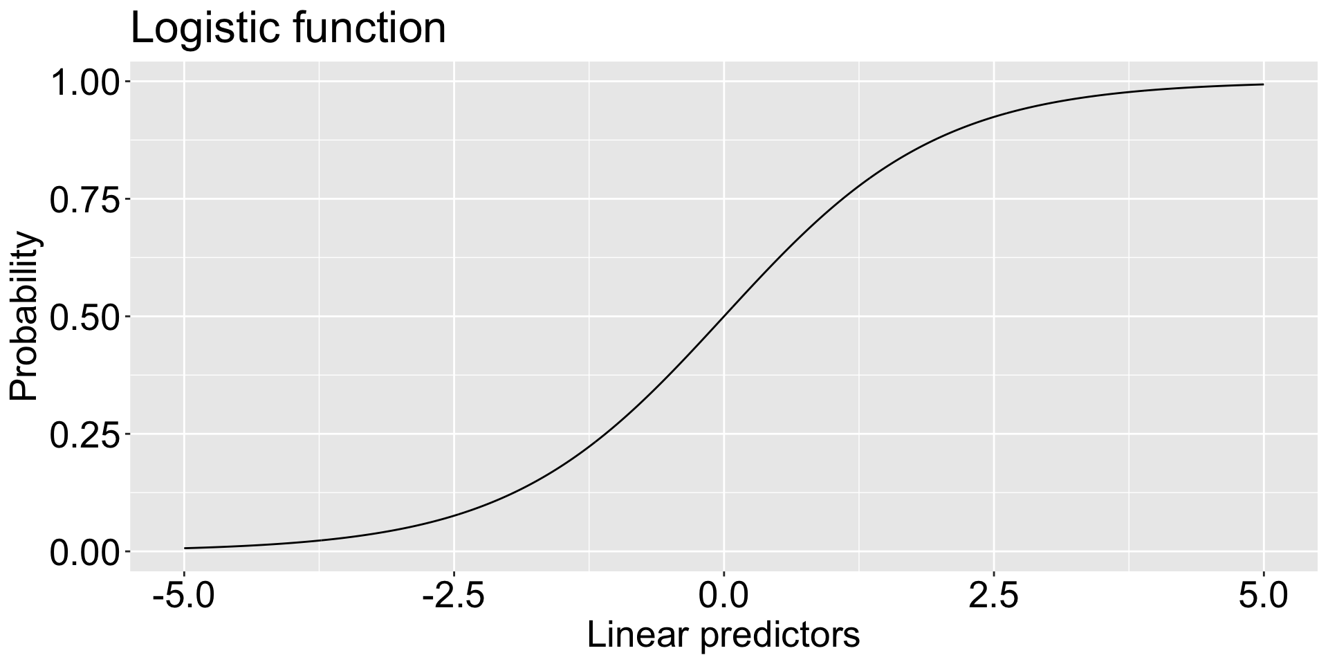
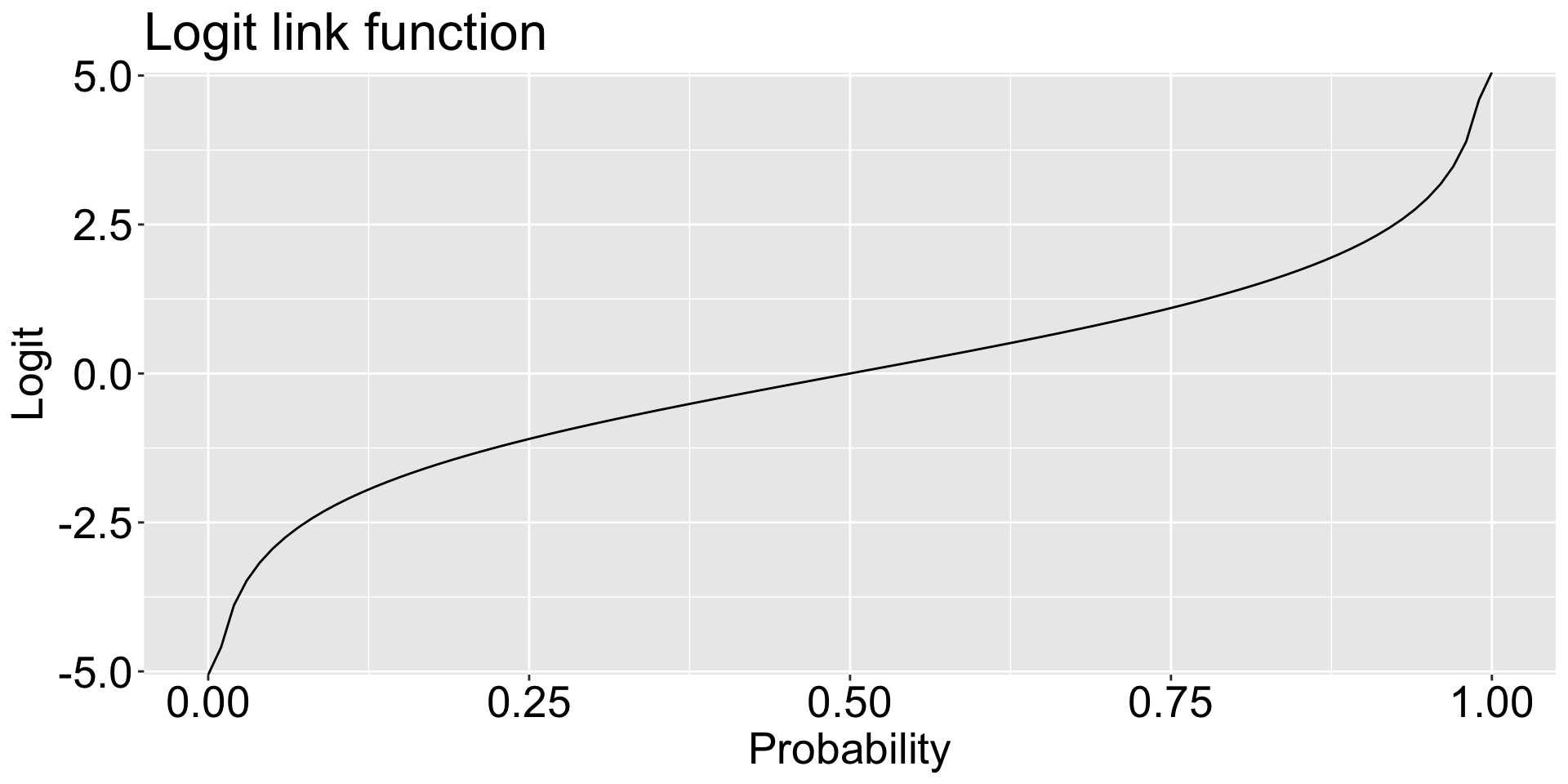
type = "link" gives the prediction of the linear predictors: (-Inf, Inf)

pred_link <- predict(mod1, type = "link") 
head(pred_link, 4)

         1          2          3          4 
 0.6398517  0.3126680 -2.0567488 -1.3138332 

type = "response" gives the prediction of the odds/ probability: [0, 1]

pred_response <- predict(mod1, type = "response")
head(pred_response, 4)

        1         2         3         4 
0.6547199 0.5775364 0.1133722 0.2118461 

If we take the prediction in probability and convert it with the log-odds function, \(\log \frac{p}{1-p}\), we get the prediction in linear predictors:

log(pred_response[1:4] /(1 - pred_response[1:4]))

         1          2          3          4 
 0.6398517  0.3126680 -2.0567488 -1.3138332 

Example: Predictions from logistic models

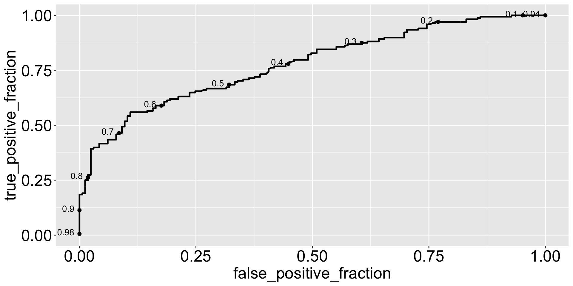
How should we decide where to cut off the predicted probabilities to classify sex?

• A reasonable choice is 0.5: if predicted probability > 0.5, classify as male (1); otherwise female (0)

penguins_pred <- penguins_clean |> 
  select(species, bill_len:sex) |> 
  mutate(pred = predict(mod1, type = "response"),
         class = ifelse(pred > 0.5, 1, 0)) 
head(penguins_pred, 5)

# A tibble: 5 × 8
  species bill_len bill_dep flipper_len body_mass   sex  pred class
  <fct>      <dbl>    <dbl>       <int>     <int> <dbl> <dbl> <dbl>
1 Adelie      39.1     18.7         181      3750     1 0.655     1
2 Adelie      39.5     17.4         186      3800     0 0.578     1
3 Adelie      40.3     18           195      3250     0 0.113     0
4 Adelie      36.7     19.3         193      3450     0 0.212     0
5 Adelie      39.3     20.6         190      3650     1 0.383     0

In R, for factor variable with two levels, first level is treated as the reference category, which corresponds to 0.

levels(penguins$sex)

[1] "female" "male"  

Example: Classification metrics

Then we can calculate the number of correct and incorrect predictions:

library(caret)
res <- confusionMatrix(
    reference = as.factor(penguins_pred$sex),
    data = as.factor(penguins_pred$class))
res$table

          Reference
Prediction   0   1
         0 112  54
         1  53 114

This is called a confusion matrix.

• True Positive (TP): 112 (really positive)
• True Negative (TN): 114 (really negative)
• False Positive (FP): 53 (fake positive - predicted positive but actually negative)
• False Negative (FN): 54 (fake negative - predicted negative but actually positive)

Positive and negative are relevant to the prediction.

Example: Classification metrics

When we assign p > 0.5 as male (1):

res$table

          Reference
Prediction   0   1
         0 112  54
         1  53 114

• Accuracy: (TP + TN) / (TP + TN + FP + FN):
  • (112 + 114) / (112 + 114 + 54 + 53) = 0.6786787
  • 67% of the prediction is correct.
• false positive rate : the proportion of positive (1) among all the reference = 0
  • 53/ (112 + 53) = 0.32
  • In the 165 female penguins, there are 32% mis-diagnosed.
• true positive rate: the proportion of positive (1) among all the reference = 1
  • 114 / (114 + 54) = 0.6786
  • In the 168 male penguins, we identified 67% of them correctly.

Example: Classification metrics

What would happen if we change the cutoff value for \(p\) to predict male/ female?

Cut off at 0.4:

          Reference
Prediction female male
    female     91   37
    male       74  131

Accuracy:

• (91 + 131) / (91 + 131 + 37 + 74) = 0.66

• about the same

false positive rate: 74 / (74 + 91) = 0.44 - worse

true positive rate: 131 / (131 + 37) = 0.77 - better

Cut off at 0.7:

          Reference
Prediction female male
    female    151   91
    male       14   77

Accuracy:

(151 + 77) / (151 + 77 + 91 + 14) = 0.68

about the same

false positive rate: 14 / (14 + 151) = 0.08 - better

true positive rate: 77 / (77 + 91) = 0.45 - worse

Example: ROC curve

penguins_clean |> 
  mutate(pred = predict(mod1, type = "response")) |> 
  ggplot() + 
  geom_roc(aes(m = pred, d = sex), cutoffs.at = seq(0,1, 0.1), labelround = 2) 

m refers to the continous Measurement and d refers to the binary Diagnosis (not necessarily the best naming).

The ROC curve shows the trade-off between true positive rate and false positive rate at different threshold values.

Is this a good model?

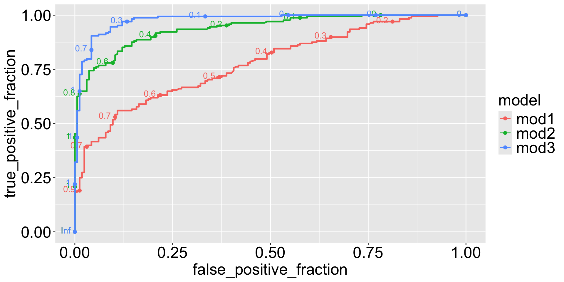
Example: Model comparison

mod2 <- glm(sex ~ body_mass + flipper_len + species,  family = binomial,
            data = penguins_clean)
mod3 <- glm(sex ~ body_mass + flipper_len + bill_len + bill_dep + species, 
            family = binomial, data = penguins_clean)

Model 3 is the best among the three.

Example: Model comparison

summary(mod3)

(Dispersion parameter for binomial family taken to be 1)

    Null deviance: 461.61  on 332  degrees of freedom
Residual deviance: 127.11  on 326  degrees of freedom
AIC: 141.11

Number of Fisher Scoring iterations: 7

The summary seems to be different from linear models (mod0):

summary(mod0)

Residual standard error: 0.4387 on 330 degrees of freedom
Multiple R-squared:  0.237, Adjusted R-squared:  0.2324 
F-statistic: 51.26 on 2 and 330 DF,  p-value: < 2.2e-16

Why we care about deviance in logistic?

Example: Model comparison

• Deviance measures how well the model fits the data. Lower, better.

• Null deviance represents the deviance of a model with only an intercept (no predictors).

• Residual deviance represents the deviance of the fitted model with predictors.

• We can compare models using deviance: a significant reduction in deviance when adding predictors indicates that the predictors improve the model fit.

# A tibble: 3 × 4
  model null.deviance deviance   AIC
  <chr>         <dbl>    <dbl> <dbl>
1 1              462.     372.  378.
2 2              462.     207.  217.
3 3              462.     127.  141.

anova(mod1, mod2, mod3, test = "Chisq")

Analysis of Deviance Table

Model 1: sex ~ body_mass + flipper_len
Model 2: sex ~ body_mass + flipper_len + species
Model 3: sex ~ body_mass + flipper_len + bill_len + bill_dep + species
  Resid. Df Resid. Dev Df Deviance  Pr(>Chi)    
1       330     371.98                          
2       328     206.70  2  165.277 < 2.2e-16 ***
3       326     127.11  2   79.596 < 2.2e-16 ***
---
Signif. codes:  0 '***' 0.001 '**' 0.01 '*' 0.05 '.' 0.1 ' ' 1