Elements of Data Science
SDS 322E
H. Sherry Zhang
Department of Statistics and Data Sciences
The University of Texas at Austin
Fall 2025
Department of Statistics and Data Sciences
The University of Texas at Austin
Fall 2025
Learning objective
- Apply linear regression in R with the
lm()function:summary(),predict(),resid(),coef(),fitted()
- Interpret the model output and compare among models
- coefficients of multiple linear regression: numerical variables, factor variables, variable interactions
- Compare among multiple linear regression models: R squared, Adjusted R squared, AIC and BIC.
A naive machine learning task
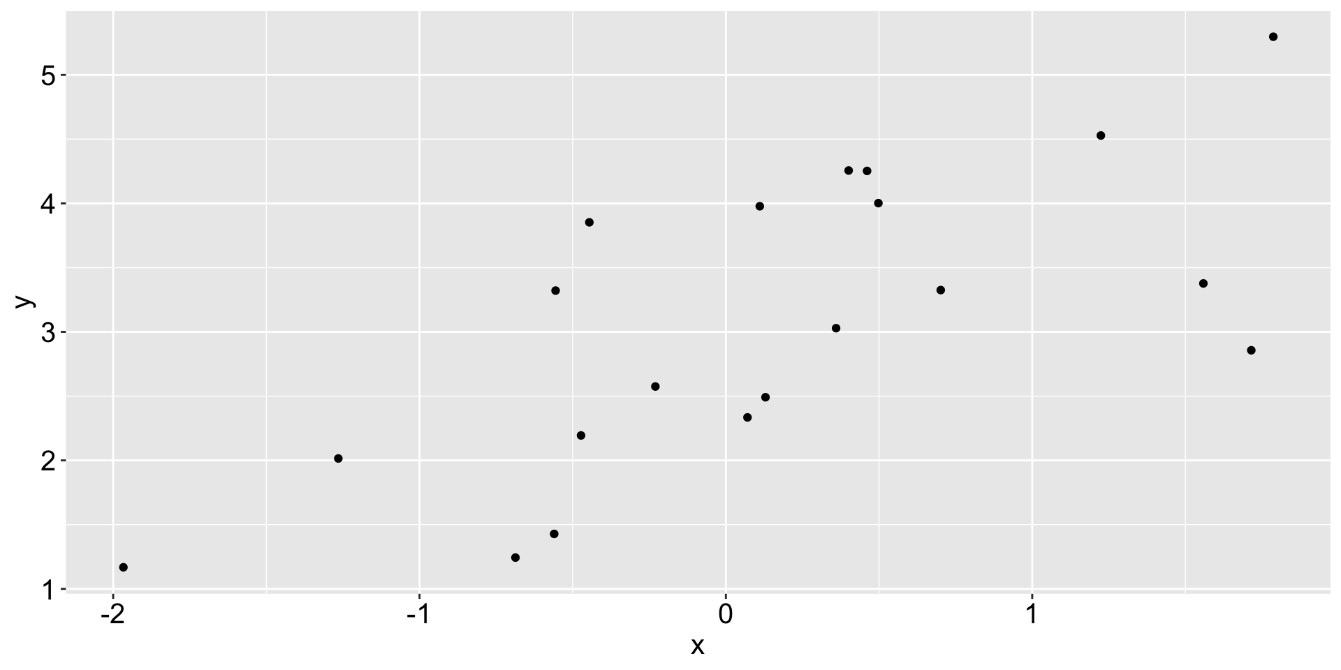
20 observations of \((x, y)\)
A lazy attempt to describe the relationship between x and y
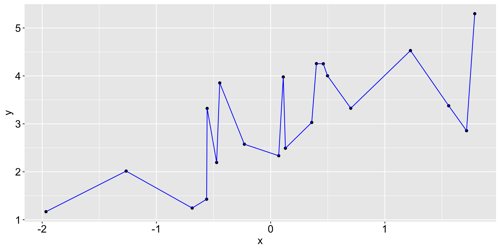
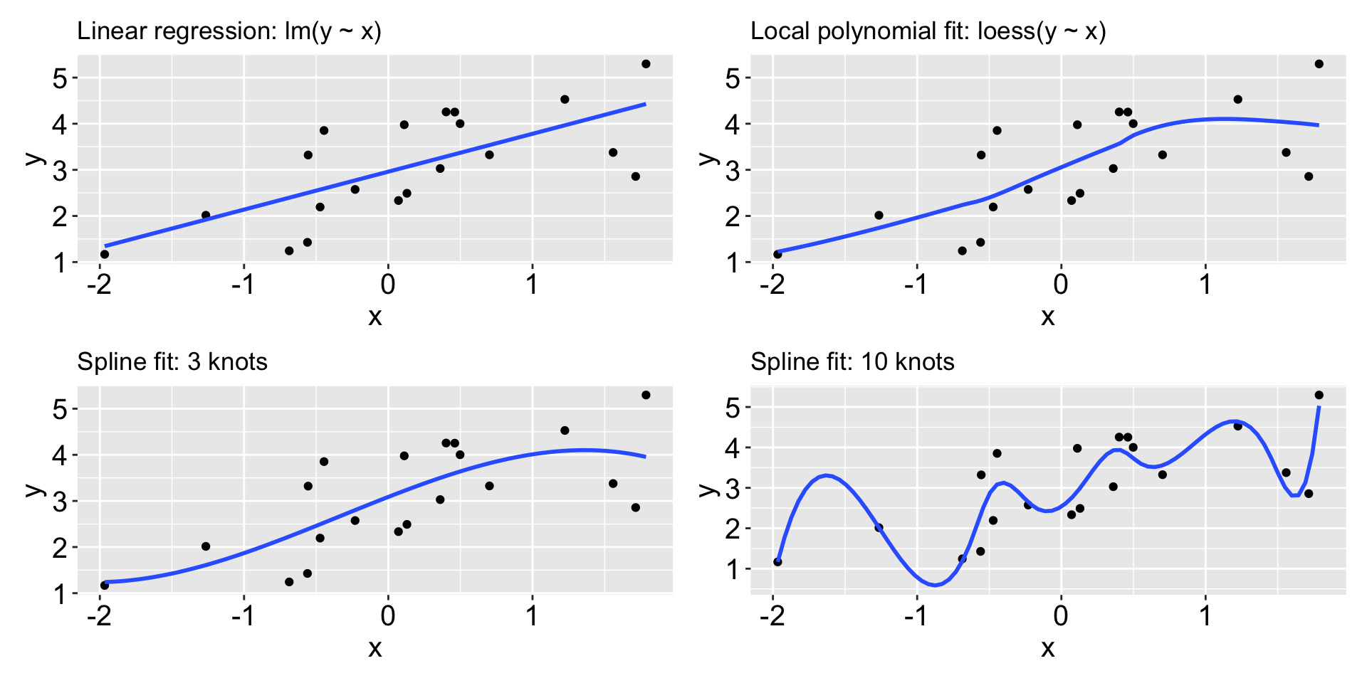
A naive machine learning task
More attempts to describe the relationship between x and y:
What does machine learning algorithms do?
Once we have a model fit, for a new observation of x, we can
- make a prediction of the
yvariable (regression) - specifically, when the
yvariable is categorical, this is called classification
What model we should use to fit the data?
- parametric models assume a specific functional form: e.g.
- linear regression: \(y = \beta_0 + \beta_1 x_1\)
- logistic regression: \(\text{logit}(P(y=1)) = \beta_0 + \beta_1 x_1\)
- non-parametric models make fewer assumptions about the functional form, e.g.
- k-nearest neighbors
- decision trees
- random forests
What does machine learning algorithms do?
Which model is the best? We need metrics to compare models:
- regression: MSE, RMSE, MAE, R squared, AIC, BIC, …
- classification: accuracy, precision, recall, F1 score, AUC, ROC…
Should we always pursue the model with the best fit? No, a model that fits well may not generalize well to new data (the issue of overfitting). What should we do then?
- train-test split: separate the data into training and testing sets to evaluate model performance on unseen data.
- there are more sophisticated method called cross-validation
All of these falls into the umbrella of supervised learning: we have the response variable y to supervise the model estimation, as opposed to the unsupervised learning where we only have the x variables (clustering, dimension reduction).
Linear regression
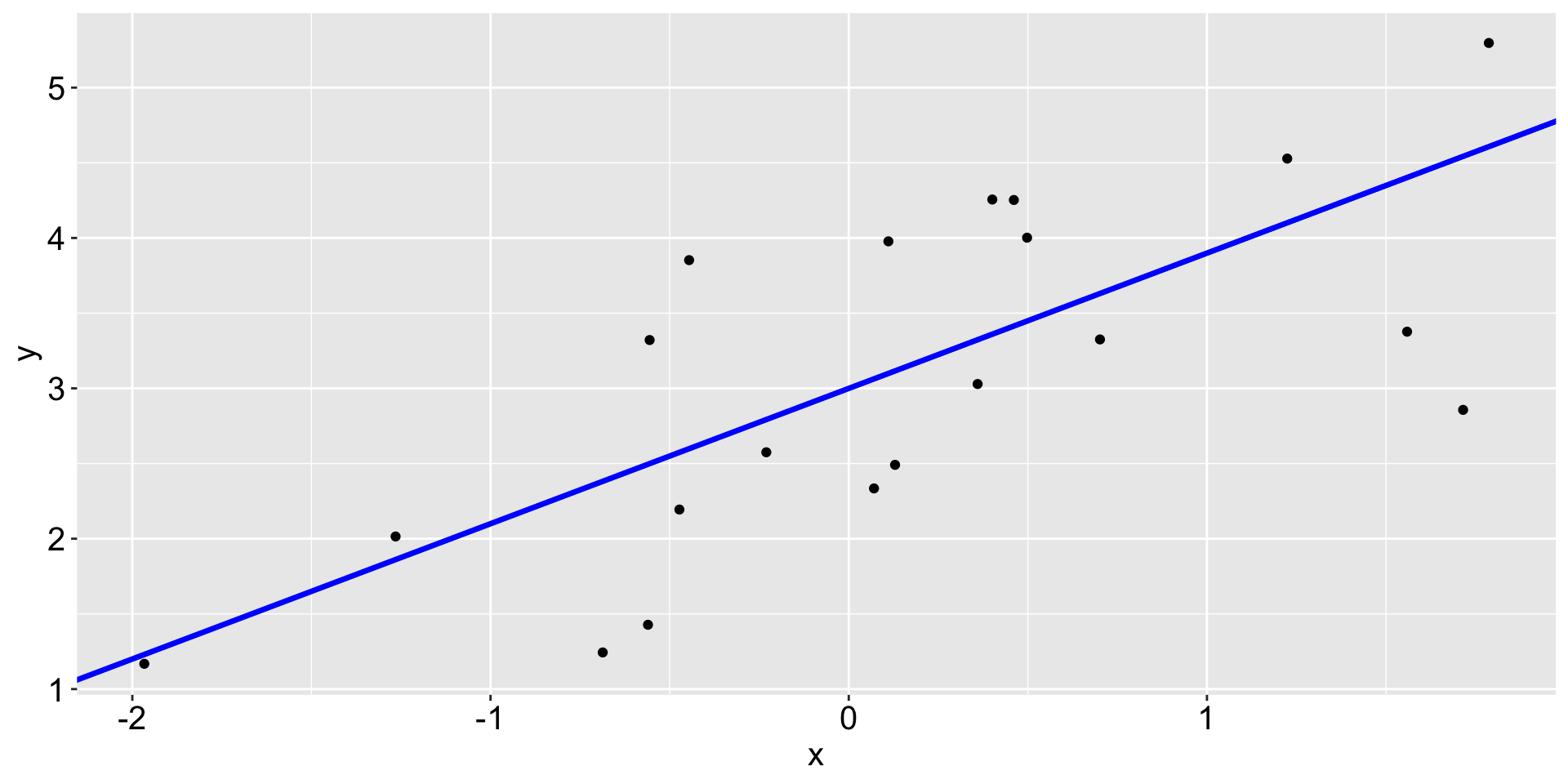
The black points are the original data and the blue line is called a fit.
Linear regression
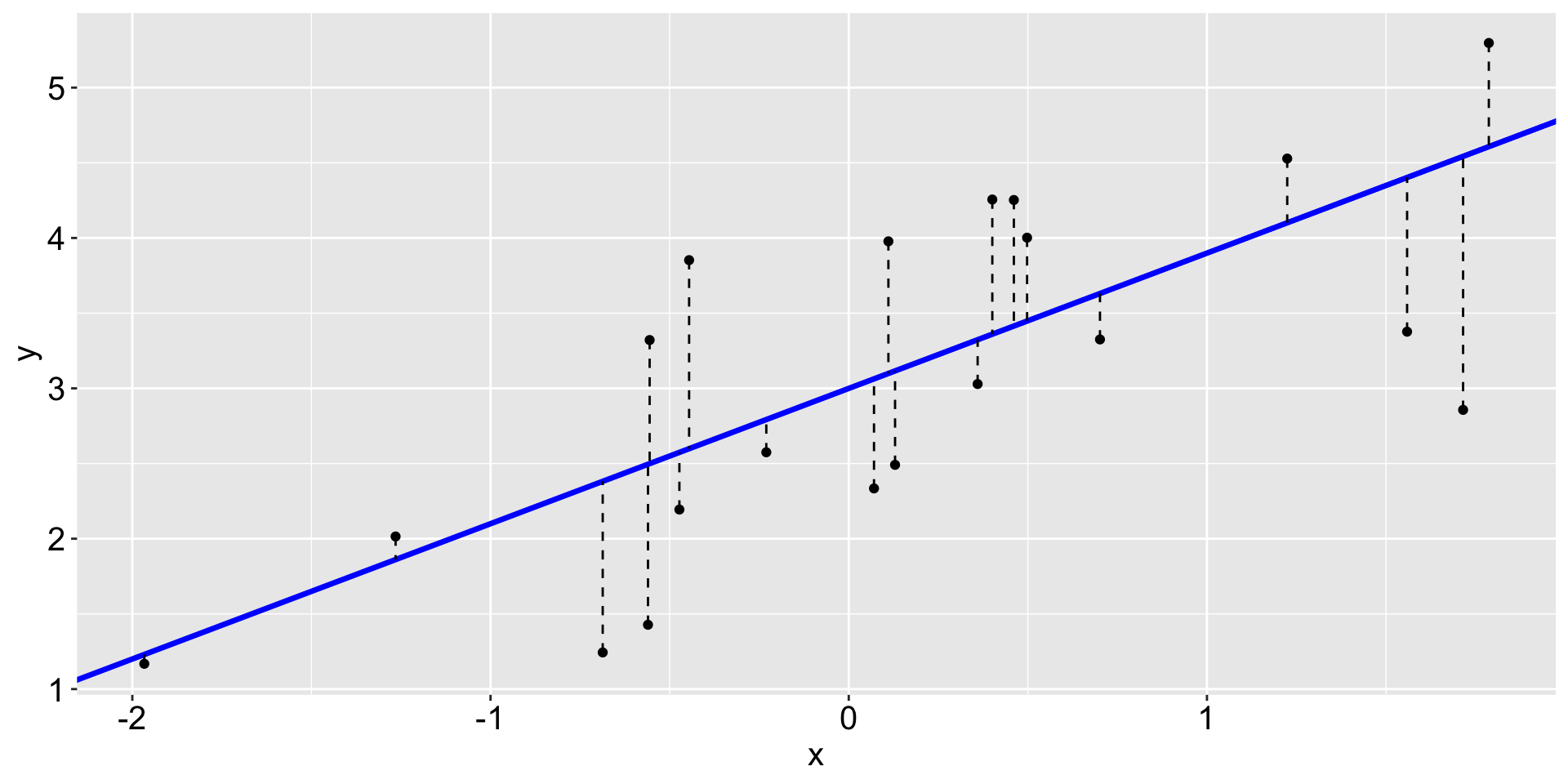
The dashed lines are called residuals.
Linear regression
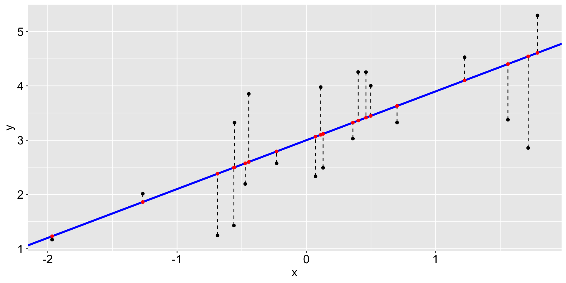
The red points on the fitted line are the fitted values or predicted values.
Why the blue line in particular?
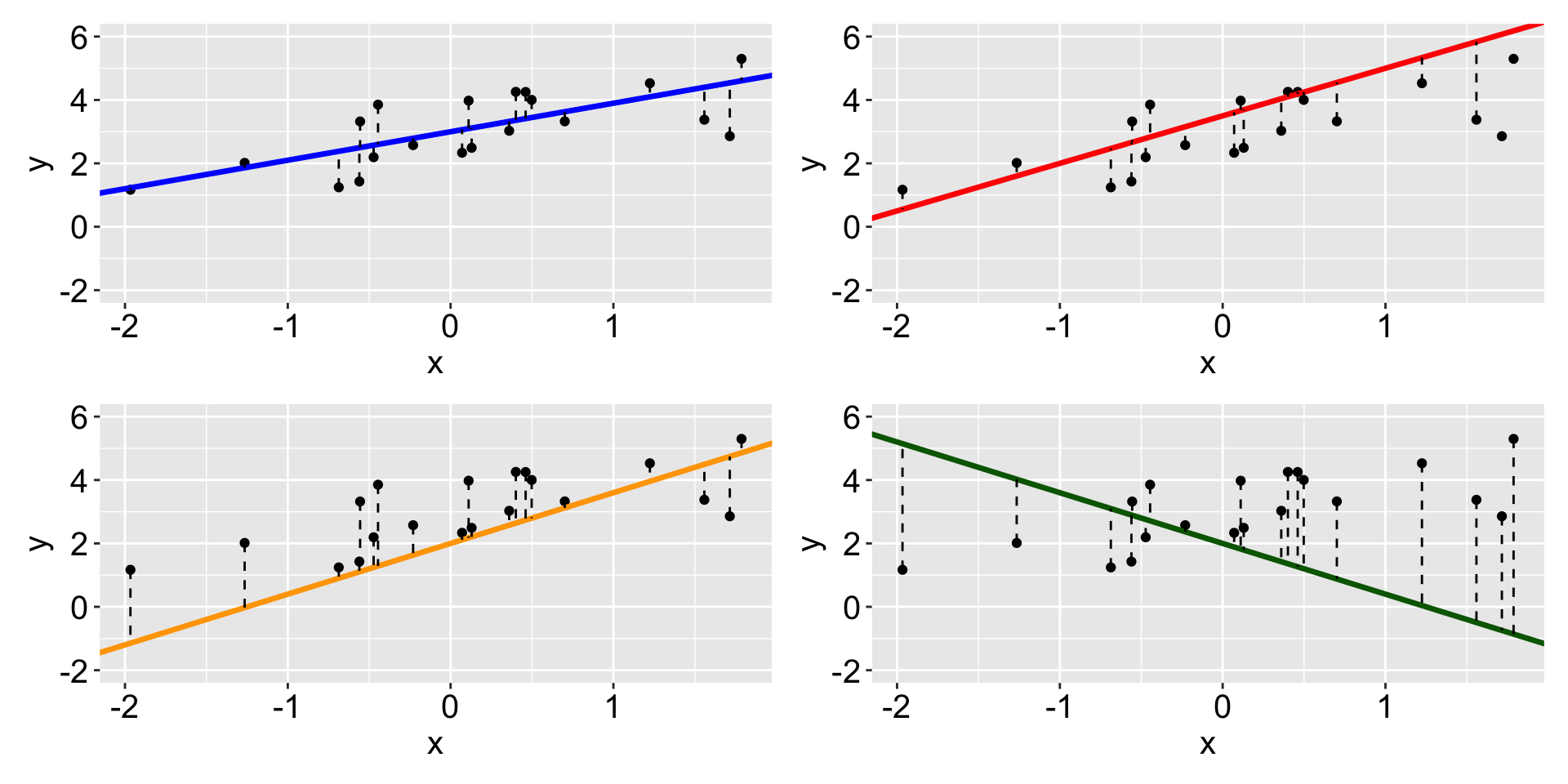
Linear regression produces a linear fit (blue) that minimize the sum of square of residuals.
Linear regression in R (Part I)
Use the
lm()function to obtain the linear regression fit.Use
predict()to get the fitted valueUse
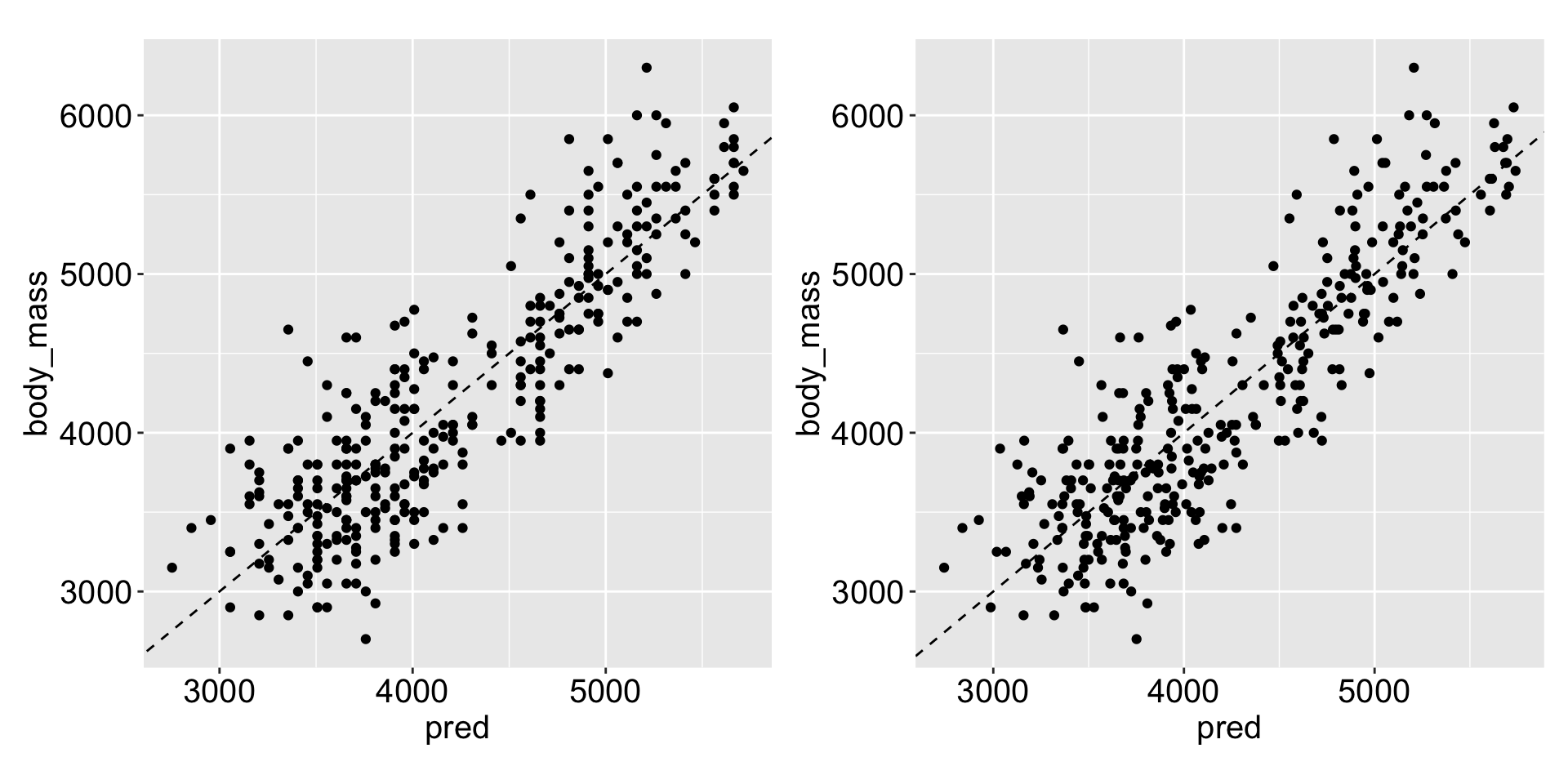
resid()to check the residualPlot the fitted value against the original data to view the fit
Example: Penguins data
Follow along the class example with
usethis::create_from_github(SDS322E-2025Fall/1002-linear")
# A tibble: 333 × 8
   species island    bill_len bill_dep flipper_len body_mass sex     year
   <fct>   <fct>        <dbl>    <dbl>       <int>     <int> <fct>  <int>
 1 Adelie  Torgersen     39.1     18.7         181      3750 male    2007
 2 Adelie  Torgersen     39.5     17.4         186      3800 female  2007
 3 Adelie  Torgersen     40.3     18           195      3250 female  2007
 4 Adelie  Torgersen     36.7     19.3         193      3450 female  2007
 5 Adelie  Torgersen     39.3     20.6         190      3650 male    2007
 6 Adelie  Torgersen     38.9     17.8         181      3625 female  2007
 7 Adelie  Torgersen     39.2     19.6         195      4675 male    2007
 8 Adelie  Torgersen     41.1     17.6         182      3200 female  2007
 9 Adelie  Torgersen     38.6     21.2         191      3800 male    2007
10 Adelie  Torgersen     34.6     21.1         198      4400 male    2007
# ℹ 323 more rowsExample: Penguins data
We can use summary() to look at the result: summary(mod1)
Call:
lm(formula = body_mass ~ flipper_len, data = penguins_clean)

Residuals:
     Min       1Q   Median       3Q      Max
-1057.33  -259.79   -12.24   242.97  1293.89

Coefficients:
            Estimate Std. Error t value Pr(>|t|)
(Intercept) -5872.09     310.29  -18.93   <2e-16 ***
flipper_len    50.15       1.54   32.56   <2e-16 ***
---
Signif. codes:  0 '***' 0.001 '**' 0.01 '*' 0.05 '.' 0.1 ' ' 1

Residual standard error: 393.3 on 331 degrees of freedom
Multiple R-squared:  0.7621,    Adjusted R-squared:  0.7614
F-statistic: 1060 on 1 and 331 DF, p-value: < 2.2e-16Interpretation: If flipper length to increase 1 mm, we would expect the penguins body mass to crease 50.15 grams.
Here we can read the coefficient as 50.15, how can we access it? How can we access the predicted value? How can we access the residuals?
Example: penguins data - function design
You may already know that we can assess those information from res$coefficients, res$fitted.values, and res$residuals. But there are also functions like coef(res), predicted(res)/ fitted(res), and resid(res). Why bother?
You can directly assess them with easy models (like
lm):res$fitted.values, while others may need additional computation, for example as we will see in logistic regression. This meansres$fitted.valuesbut this won’t work for aglmobject.By using a function
fitted(), we can define how we would like the fitted value to be computed for each type of object (lmorglmor others). Then we can always use the same syntaxfitted(res)to obtain the fitted values for both cases.
- This is the idea behind object-oriented programming. In the language of OOP,
lm,glmare called classesfitted(),coef()are called generics (they are S3 generics).- When a generic is called, R uses method dispatch to call the corresponding method for each class:
coef.lm(),coef.glm()(they are hidden).
Example: penguins data
R squared: the proportion of the variance in y that is predictable from the xs in a regression model. Larger, better.
Adjusted R squared: give penalty for including more variables. Larger, better.
 [1] "call"          "terms"         "residuals"     "coefficients"
 [5] "aliased"       "sigma"         "df"            "r.squared"
[9] "adj.r.squared" "fstatistic" "cov.unscaled" Do you think we can make this model better? What other information you may want to include to predict the penguin weight?
# A tibble: 5 × 8
  species island    bill_len bill_dep flipper_len body_mass sex     year
  <fct>   <fct>        <dbl>    <dbl>       <int>     <int> <fct>  <int>
1 Adelie  Torgersen     39.1     18.7         181      3750 male    2007
2 Adelie  Torgersen     39.5     17.4         186      3800 female  2007
3 Adelie  Torgersen     40.3     18           195      3250 female  2007
4 Adelie  Torgersen     36.7     19.3         193      3450 female  2007
5 Adelie  Torgersen     39.3     20.6         190      3650 male    2007
Example: penguins data
I can think of a few. We may want to include
- other numerical variables:
bill_lenandbill_dep - other categorical variables:
speciesandsex - interactions of these variables
- numerical x numerical
- numerical x categorical
- categorical x categorical
- …
Example: penguins data - multiple linear regression
Include more numerical variables:
mod <- lm(body_mass ~ flipper_len + bill_len + bill_dep, data = penguins_clean)
summary(mod)$r.squared
[1] 0.7639367Previously
Does it improve our model much?
Multiple linear regression - factor variables
Include factor variables:
               Estimate Std. Error    t value      Pr(>|t|)
(Intercept) -5410.30022 285.797694 -18.930524  1.252078e-54
flipper_len    46.98218   1.441257  32.598066 3.329486e-105
sexmale       347.85025  40.341557   8.622628  2.781882e-16
Interpretation: Holding flipper length constant, male penguins are on average 347.85 grams heavier than female penguins.
- The coefficient measures the difference between
maleto the base level (femalehere).
Why we only estimate one coefficient for sexmale?
- Include both
sexmaleandsexfemalewould create perfect multicollinearity: when computing the OLS estimator: \((X^TX)^{-1}X^Ty\), \(X^TX\) becomes singular, hence can’t calculate its inverse and the OLS estimator is undefined.
Multiple linear regression - factor variables
How can we change the reference level from female to male?
penguins_clean2 <- penguins_clean |> mutate(sex = fct_relevel(sex, c("male", "female")))
lm(body_mass ~ flipper_len + sex, data = penguins_clean2) |> summary() |> coef()
Estimate Std. Error t value Pr(>|t|)
(Intercept) -5062.44997 296.021652 -17.101621 2.141396e-47
flipper_len 46.98218 1.441257 32.598066 3.329486e-105
sexfemale -347.85025 40.341557 -8.622628 2.781882e-16Previously
This interpretation extrapolates for factor variables with more than two levels.
                    Estimate Std. Error   t value     Pr(>|t|)
(Intercept)      -4013.17889 586.245983 -6.845555 3.740845e-11
flipper_len         40.60617   3.079553 13.185734 3.642114e-32
speciesChinstrap  -205.37548  57.566442 -3.567625 4.137585e-04
speciesGentoo      284.52360  95.430335  2.981480 3.082533e-03
Multiple linear regression - compare among models
# A tibble: 4 × 6
  model r.squared adj.r.squared logLik   AIC   BIC
  <chr>     <dbl>         <dbl>  <dbl> <dbl> <dbl>
1 1         0.762         0.761 -2461. 4928. 4940.
2 2         0.806         0.805 -2427. 4862. 4878.
3 3         0.787         0.785 -2443. 4895. 4914.
4 4         0.867         0.865 -2364. 4741. 4764.
Which model is the best? What criteria would you use to compare these models?
r.squared(adj.r.squared): variance explained (with penalty).AIC(Akaike Information Criterion) andBIC(Bayesian Information Criterion): penalize model complexity. Lower, better. AIC = \(2k - 2ln(L)\), BIC = \(ln(n)k - 2ln(L)\), where \(k\) is the number of parameters, n is the number of observations, and \(L\) is the maximized value of the likelihood function for the model.
In all the measures, mod4 is the best.
Multiple linear regression - interaction terms
Do you think for each species, the gender difference of body mass is different? e.g. For Gentoo, would the difference between male and female larger than that of Adelie?
                           Estimate Std. Error    t value     Pr(>|t|)
(Intercept)              -478.33627 528.705254 -0.9047314 3.662758e-01
flipper_len                20.48607   2.809638  7.2913556 2.341573e-12
sexmale                   580.08485  49.295738 11.7674442 6.993322e-27
speciesChinstrap           77.63930  60.676659  1.2795579 2.016106e-01
speciesGentoo             800.54906  86.334124  9.2726841 2.567726e-18
sexmale:speciesChinstrap -335.82390  84.959856 -3.9527362 9.477863e-05
sexmale:speciesGentoo      44.03410  71.965611  0.6118770 5.410456e-01
Interpretation:
The coefficient of
speciesGentoois 800.54, meaning that holding flipper length constant, the body mass of female Gentoo penguins is on average 800.54 grams lighter than that of female Adelie penguins (baseline).The coefficient of
sexmale:speciesGentoois 44.03, meaning that holding flipper length constant, the gender difference of body mass for Gentoo penguins is 44.03 grams heavier than that of Adelie penguins.
Multiple linear regression - interaction terms
Multiple linear regression - interaction terms
How do you calculate the body mass difference of male penguins between Gentoo and male Chinstrap (with a given flipper length)?
                           Estimate Std. Error    t value     Pr(>|t|)
(Intercept)              -478.33627 528.705254 -0.9047314 3.662758e-01
flipper_len                20.48607   2.809638  7.2913556 2.341573e-12
sexmale                   580.08485  49.295738 11.7674442 6.993322e-27
speciesChinstrap           77.63930  60.676659  1.2795579 2.016106e-01
speciesGentoo             800.54906  86.334124  9.2726841 2.567726e-18
sexmale:speciesChinstrap -335.82390  84.959856 -3.9527362 9.477863e-05
sexmale:speciesGentoo      44.03410  71.965611  0.6118770 5.410456e-01
\[\text{body mass} = \beta_0 + \beta_1 * \text{flipper length} + \beta_2 * \text{male} + \beta_3 * \text{Chinstrap} + \newline \beta_4 * \text{Gentoo} + \beta_5 * \text{male: Chinstrap} + \beta_6 * \text{male: Gentoo}\]
- Male Gentoo: \(\beta_0 + \beta_1 * \text{flipper length} + \beta_2 + \beta_4 + \beta_6\)
- Male Chinstrap: \(\beta_0 + \beta_1 * \text{flipper length} + \beta_2 + \beta_3 + \beta_5\)
- Difference: \((\beta_4 + \beta_6) - (\beta_3 + \beta_5) = 800.54 + 44.03 - (77.63 - 335.82) = 1102.76\)
Multiple linear regression - interaction terms
We can also change the reference level for both sex and species: male and Chinstrap as reference
mod6 <- lm(
  body_mass ~ flipper_len + sex * species,
  data = penguins_clean |>
    mutate(sex = fct_relevel(sex, c("male", "female")),
           species = fct_relevel(species, c("Chinstrap", "Gentoo", "Adelie"))))
summary(mod6) |> coef()
Estimate Std. Error t value Pr(>|t|)
(Intercept) -156.43602 563.837087 -0.277449 7.816112e-01
flipper_len 20.48607 2.809638 7.291356 2.341573e-12
sexfemale -244.26095 73.376078 -3.328891 9.717266e-04
speciesGentoo 1102.76776 86.455578 12.755311 1.667545e-30
speciesAdelie 258.18460 63.270856 4.080624 5.653285e-05
sexfemale:speciesGentoo -379.85800 87.387054 -4.346845 1.848112e-05
sexfemale:speciesAdelie -335.82390 84.959856 -3.952736 9.477863e-05Now we can directly read the difference of male penguins between Gentoo and Chinstrap from the coefficient of speciesGentoo: 1102.76 grams.
Multiple linear regression - interaction terms
More on the syntax:
lm(body_mass ~ flipper_len + sex * species, data = penguins_clean)
is equivalent to
lm(body_mass ~ flipper_len + sex + species + sex:species, data = penguins_clean)
Would it be a good idea to only include the interaction term sex:species without the main effects sex and species?
No…
Should we include interaction terms in our model?
# A tibble: 5 × 5
  call                                    r.squared adj.r.squared   AIC   BIC
  <chr>                                       <dbl>         <dbl> <dbl> <dbl>
1 body_mass ~ flipper_len                     0.762         0.761 4928. 4940.
2 body_mass ~ flipper_len + sex               0.806         0.805 4862. 4878.
3 body_mass ~ flipper_len + species           0.787         0.785 4895. 4914.
4 body_mass ~ flipper_len + sex + species     0.867         0.865 4741. 4764.
5 body_mass ~ flipper_len + sex * species     0.875         0.873 4724. 4754.
Multiple linear regression - interaction terms
ANOVA test: check if including the interaction terms significantly improve the model fit:
Analysis of Variance Table

Model 1: body_mass ~ flipper_len + sex + species
Model 2: body_mass ~ flipper_len + sex * species
  Res.Df      RSS Df Sum of Sq      F    Pr(>F)
1    328 28653568
2    326 26913579  2   1739989 10.538 3.675e-05 ***
---
Signif. codes:  0 '***' 0.001 '**' 0.01 '*' 0.05 '.' 0.1 ' ' 1
Is it always the case that we should include interaction term?
penguins_small <- penguins_clean |> group_by(species) |> slice_sample(n = 10) |> ungroup()
mod14 <- lm(body_mass ~ flipper_len + sex + species, data = penguins_small)
mod15 <- lm(body_mass ~ flipper_len + sex * species, data = penguins_small)
anova(mod14, mod15)
Analysis of Variance Table
Model 1: body_mass ~ flipper_len + sex + species
Model 2: body_mass ~ flipper_len + sex * species
Res.Df RSS Df Sum of Sq F Pr(>F)
1 25 2000604
2 23 1824245 2 176359 1.1118 0.346Multiple linear regression: interaction term is never gonna end
How about categorical x numerical interaction?
mod7 <- lm(body_mass ~ flipper_len + species + sex * bill_len, data = penguins_clean)
summary(mod7) |> coef()
Estimate Std. Error t value Pr(>|t|)
(Intercept) -1279.18353 601.073136 -2.128166 3.407308e-02
flipper_len 19.05161 2.954206 6.448980 4.061426e-10
speciesChinstrap -302.26775 81.331367 -3.716497 2.376640e-04
speciesGentoo 670.46914 95.795308 6.998977 1.474486e-11
sexmale 1004.94633 279.166183 3.599814 3.679467e-04
bill_len 28.69485 7.980449 3.595644 3.736613e-04
sexmale:bill_len -12.52461 6.403327 -1.955953 5.132445e-02Interpretation:
- the coefficient for
bill_len(28.695): Holding flipper length and species constant, for female penguins, for each additional mm in bill length, body mass is expected to increase by 28.695 grams on average. (the effect of female penguins)
Multiple linear regression: interaction term is never gonna end
For a bill length of 40mm, what’s the difference in body mass between male and female penguins?
                    Estimate Std. Error   t value     Pr(>|t|)
(Intercept)      -1279.18353 601.073136 -2.128166 3.407308e-02
flipper_len         19.05161   2.954206  6.448980 4.061426e-10
speciesChinstrap  -302.26775  81.331367 -3.716497 2.376640e-04
speciesGentoo      670.46914  95.795308  6.998977 1.474486e-11
sexmale           1004.94633 279.166183  3.599814 3.679467e-04
bill_len            28.69485   7.980449  3.595644 3.736613e-04
sexmale:bill_len -12.52461 6.403327 -1.955953 5.132445e-02\[\text{body mass} = \beta_0 + \beta_1 * \text{flipper length} + \beta_2 * \text{Chinstrap} + \beta_3 * \text{Gentoo} + \newline \beta_4 * \text{male} + \beta_5 * \text{bill length} + \beta_6 * \text{male: bill length}\]
- male : \(\beta_0 + \beta_1 * \text{flipper length} + \beta_4 + \beta_5 * 40 + \beta_6 * 40\)
- female : \(\beta_0 + \beta_1 * \text{flipper length} + \beta_5 * 40\)
- difference: \(\beta_4 + \beta_6 * 40 = 1004.946 + -12.525 * 40 = 503.946\) grams.
Does the species matter?
Multiple linear regression: interaction term is never gonna end
Continous x continous interaction
mod8 <- lm(body_mass ~ flipper_len + species + bill_dep * bill_len, data = penguins_clean)
summary(mod8) |> coef()
Estimate Std. Error t value Pr(>|t|)
(Intercept) -8935.45352 1982.121363 -4.508025 9.136524e-06
flipper_len 20.80620 3.121097 6.666311 1.121395e-10
speciesChinstrap -449.05376 84.193033 -5.333621 1.803914e-07
speciesGentoo 877.68723 145.281214 6.041299 4.170566e-09
bill_dep 398.41075 107.560085 3.704076 2.491162e-04
bill_len 147.51625 45.041999 3.275082 1.169859e-03
bill_dep:bill_len -6.09707 2.515064 -2.424221 1.588474e-02\[\text{body mass} = \beta_0 + \beta_1 * \text{flipper length} + \beta_2 * \text{Chinstrap} + \beta_3 * \text{Gentoo} + \newline \beta_4 * \text{bill depth} + \beta_5 * \text{bill length} + \beta_6 * \text{bill depth: bill length}\]
Holding flipper length and species constant, for each additional mm in bill depth,
- At bill length of 40mm, body mass is expected to increase by (398.41 - 6.097 * 40) = 154.53 grams on average.
- At bill length of 60mm, body mass is expected to increase by (398.41 - 6.097 * 60) = 32.59 grams on average.
Other considerations: outlines, influential and leverage points
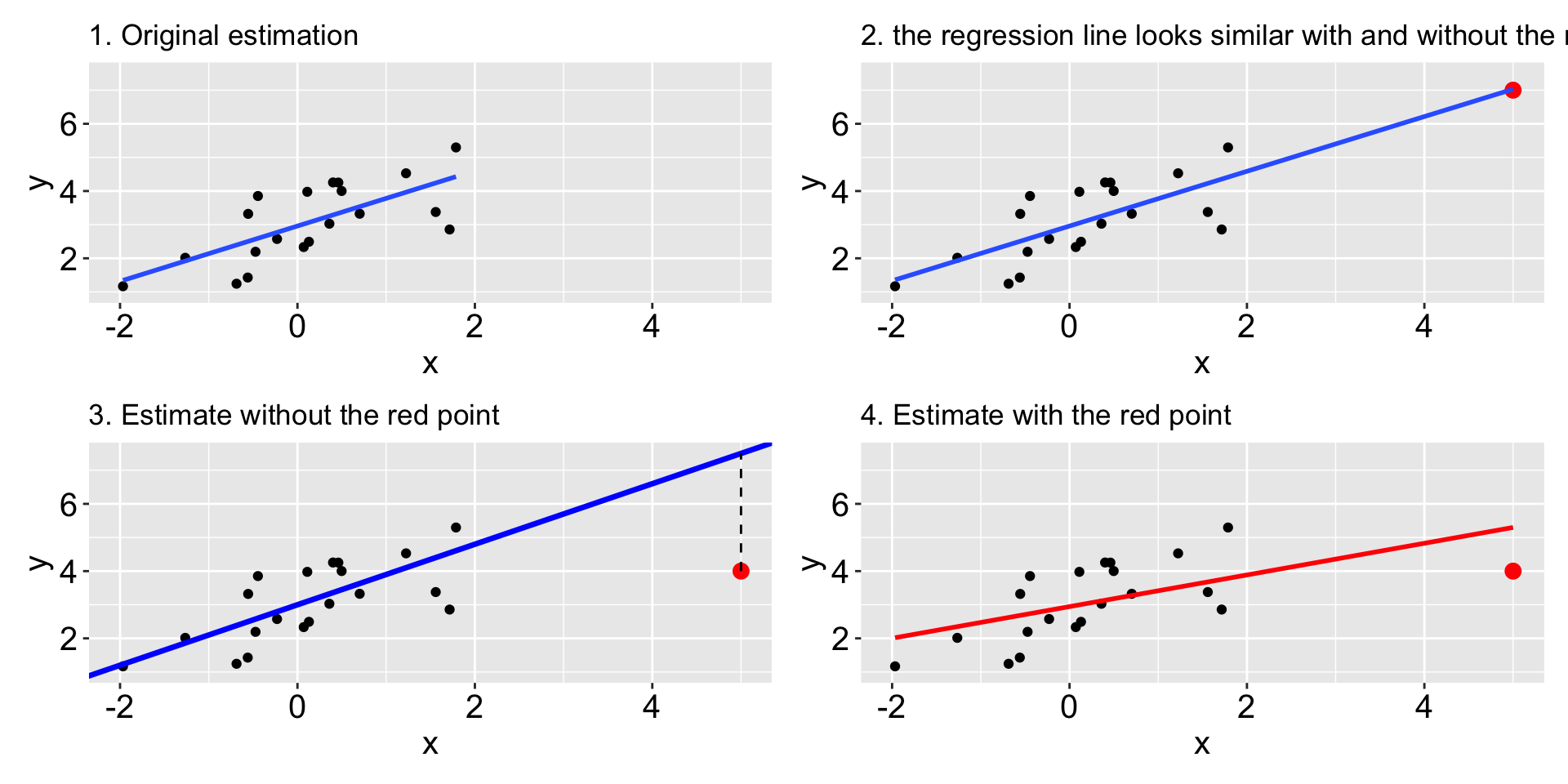
- An outlier is an individual observation with a very large residual. Shown in 3.
- An influential observation, when included, alters the regression coefficients by a meaningful amount. Shown in 4. Check Cook distance.
- leverage points: Observations that are extreme in the
xdirection are said to have high leverage - they have the potential to influence the line greatly. Shown in 2 and 3.