Elements of Data Science
SDS 322E

H. Sherry Zhang
Department of Statistics and Data Sciences
The University of Texas at Austin

Fall 2025

Learning objectives

• Understand the idea of K-nearest neighbor (KNN) classification and its computation with caret::knn3()
• Understand training-testing split and out-of-sample accuracy
• Understand the idea of cross validation for hyper-parameter selection
  • We will implement them in tidymodels on Friday

KNN

x	-5	-3	-1	0	1	2	3	4	6	8	9	10	12	15
y	1	1	1	1	1	1	0	1	0	1	0	0	0	0

Previously from a logistic regression

for x = 3.5, y = 0.72, predict 1.

Maybe there are other things to make a prediction …

How about lets like the 3 points that are closest to x = 3.5:

x	2	3	4
y	1	0	1

What’s the “average”/ majority vote?

It should get predicted to 1

This is k-nearest neighbor with k = 3.

What would you predict at x = 3 with k = 1?

Binary prediction with KNN

Follow along the class example with

usethis::create_from_github(SDS322E-2025Fall/1102-knn")

penguins_clean <- as_tibble(datasets::penguins) |> na.omit()
head(penguins_clean, 3)

# A tibble: 3 × 8
  species island    bill_len bill_dep flipper_len body_mass sex     year
  <fct>   <fct>        <dbl>    <dbl>       <int>     <int> <fct>  <int>
1 Adelie  Torgersen     39.1     18.7         181      3750 male    2007
2 Adelie  Torgersen     39.5     17.4         186      3800 female  2007
3 Adelie  Torgersen     40.3     18           195      3250 female  2007

Goal: predict sex based on bill_len and bill_dep with KNN.

Step 1: Scale the predictors with scales()

Step 2: Fit a KNN model with caret::knn3()

Step 3: Predict on the testing data

Step 4: Calculate classification metrics

Step 1: Scale the predictors

We would like to scale all the predictors (bill_len and bill_dep), but not the response variable sex:

penguins_std <- penguins_clean |> 
  select(bill_len, bill_dep) |> 
  scale() |> 
  bind_cols(sex = penguins_clean$sex)

penguins_std |> head()

# A tibble: 6 × 3
  bill_len bill_dep sex   
     <dbl>    <dbl> <fct> 
1   -0.895    0.780 male  
2   -0.822    0.119 female
3   -0.675    0.424 female
4   -1.33     1.08  female
5   -0.858    1.74  male  
6   -0.931    0.323 female

Step 2: Fit a KNN model using caret::knn3()

knn_res <- knn3(sex ~ bill_len + bill_dep,  data = penguins_std)

Exercise: What is the default number of neighbors (k) in knn3()?

• k = 5 by default.

Step 3: Predict on the standardized data

knn_pred <- predict(knn_res, newdata = penguins_std)
knn_pred |> head()

     female male
[1,]    0.2  0.8
[2,]    1.0  0.0
[3,]    0.4  0.6
[4,]    0.6  0.4
[5,]    0.2  0.8
[6,]    1.0  0.0

Which category do we predict for the first penguin?

Step 4: Calculate classification metrics

pred_knn_df <- as_tibble(knn_pred) |> mutate(class = ifelse(male > female, "male", "female"))

pred_knn_df |> head(5)

# A tibble: 5 × 3
  female  male class 
   <dbl> <dbl> <chr> 
1    0.2   0.8 male  
2    1     0   female
3    0.4   0.6 male  
4    0.6   0.4 female
5    0.2   0.8 male  

table(pred_knn_df$class, penguins_std$sex)

        
         female male
  female    146   18
  male       19  150

How do we compare the accuracy of KNN and logistic regression?

This time, we are comparing two different machine learning algorithms, rather than different specifications of the same model, like we did with linear model.

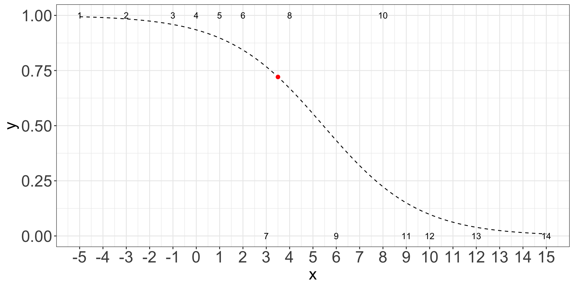
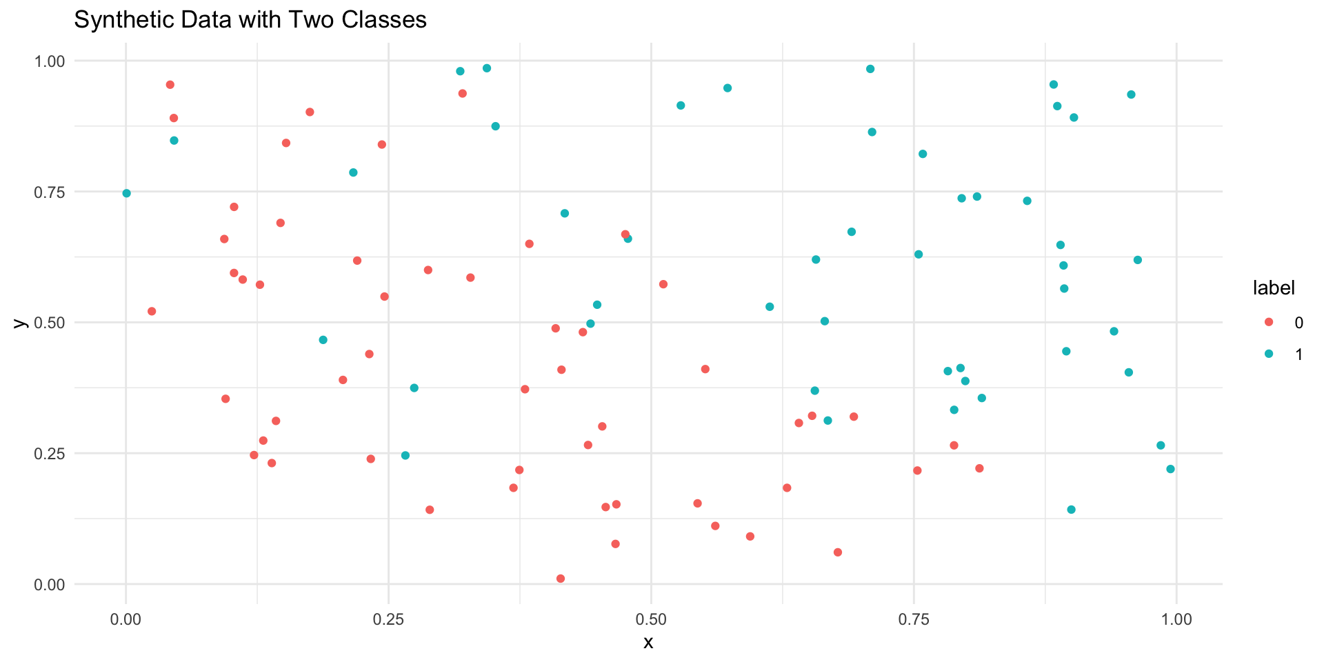
set.seed(123)
n <- 100
x <- runif(n, 0, 1)
y <- runif(n, 0, 1)
label <- ifelse(x + y + rnorm(n, 0, 0.3) > 1, 1, 0)  # add noise
data <- data.frame(x, y, label)

logit_model <- glm(label ~ x + y, data = data, family = binomial)
logit_pred <- ifelse(predict(logit_model, type = "response") > 0.5, 1, 0)
logic_acc <- mean(logit_pred == data$label)

knn_model <- knn3(label ~ x + y,  data = data, k = 7)
knn_pred <- as_tibble(predict(knn_model, newdata = data)) |> 
  mutate(class = ifelse(`0` > `1`, 0, 1)) |> 
  pull(class)
knn_acc <- mean(knn_pred == data$label)

tibble(x = x, y = y, label = factor(label)) %>%
  ggplot(aes(x = x, y = y, color = label)) +
  geom_point() +
  labs(title = "Synthetic Data with Two Classes") +
  theme_minimal()

# A tibble: 1 × 2
  logic_acc knn_acc
      <dbl>   <dbl>
1      0.83    0.86

How do we compare the accuracy of KNN and logistic regression

Why we can’t just conclude KNN is better than logistic regression because it has higher accuracy on this dataset?

• KNN is highly flexibility, we can obtain very complex decision boundary by tuning k.

A better way to evaluate the performance of different models is to evaluate their performance on unseen data.

• This is the idea behind training-testing split
• We would like to randomly split the data into a training set and a testing set. A common training/ testing ratio is 70% / 30% or 90% / 10%.

Would it be a good idea to take first two thirds of the data as training and last one third as testing?

No…

Training and testing split with logistic regression

Step 1: training-testing split (new)

m <- nrow(penguins_clean)
set.seed(123)
val <- sample(1:m, size = round(m/3), replace = FALSE)
penguins_training <- penguins_clean[-val,]
penguins_testing <- penguins_clean[val,]

Step 2: fitting the logistic regression model on the training data

mod_glm <- glm(sex ~ bill_len + bill_dep, family = binomial, data = penguins_training)

Step 3: predicting on the testing data

lr_pred_vec <- predict(mod_glm, newdata = penguins_testing, type = "response")

Step 4: calculate the classification metrics on the testing data

lr_pred_res <- tibble(pred = lr_pred_vec, pred_class = ifelse(pred > 0.5, 1, 0))
table(lr_pred_res$pred_class, penguins_testing$sex)

   
    female male
  0     43   20
  1      9   39

Your time

Can you repeat the above workflow to KNN?

Step	Description	Action / Question
1	Scale the predictors	We will do the same scaling as before
2	Training-testing split	Apply the same training testing split as the logistic regression
3	Fit KNN with the training data	How do you modify the previous fit to be on the training data?
4	Predict on the testing data	How do you modify the prediction to be on the testing data?
5	Calculate classification metrics	Can you obtain the confusion matrix from the prediction on the testing data?

Solution

# step 1
penguins_std <- penguins_clean |> 
  select(bill_len, bill_dep) |> 
  scale() |> 
  bind_cols(sex = penguins_clean$sex)

# step 2
m <- nrow(penguins_std)
set.seed(123)
val <- sample(1:m, size = round(m/3), replace = FALSE)
penguins_training <- penguins_std[-val,]
penguins_testing <- penguins_std[val,]

# step 3
knn_res <- knn3(sex ~ bill_len + bill_dep, 
                data = penguins_training)

# step 4
knn_pred <- predict(knn_res, 
                    newdata = penguins_testing)

# step 5
pred_knn_df <- as_tibble(knn_pred) |>
  mutate(class = ifelse(male > female, "male", "female"))
table(pred_knn_df$class, penguins_testing$sex)

        
         female male
  female     46   12
  male        6   47

The logistic classifier:

table(lr_pred_res$pred_class, 
      penguins_testing$sex)

   
    female male
  0     43   20
  1      9   39

Here the accuracy is out-of-sample, which is more reliable than the in-sample performance.

Visualize the space

KNN: binary response encode in numerics or factors

Would the result be different if we code the response as 0/1?

penguins_clean2 <- as_tibble(datasets::penguins) |> na.omit() |>
  mutate(sex2 = ifelse(sex == "male", 1, 0))

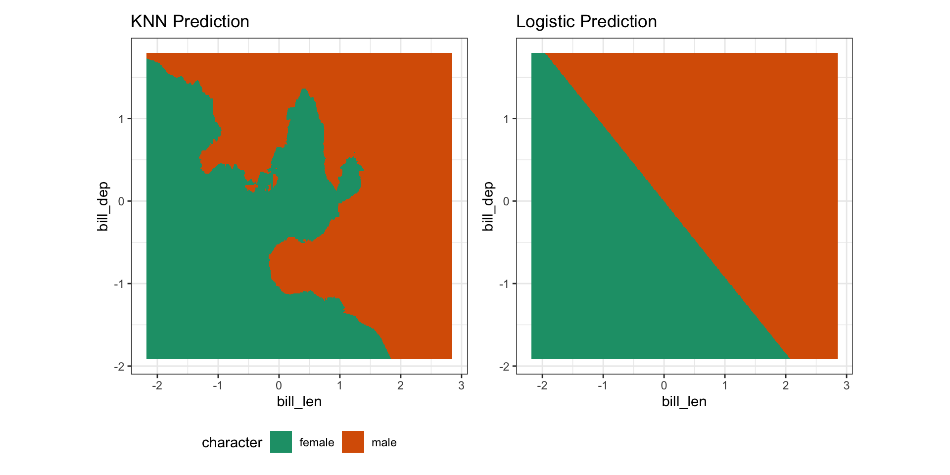
Repeat the procedure we had before and fit the KNN model and compare the prediction, specifically

• Step 1: conduct the same training testing split

• Step 2: fit the KNN model with the new sex2 as the response

• Step 3: compute the prediction and compare with the original result

Solution

# Step 1: conduct the same training testing split
penguins_std <- penguins_clean2 |> 
  select(bill_len, bill_dep) |> 
  scale() |> 
  bind_cols(sex2 = penguins_clean2$sex2)
m <- nrow(penguins_std)
set.seed(123)
val <- sample(1:m, size = round(m/3), replace = FALSE)
penguins_training2 <- penguins_std[-val,]
penguins_testing2 <- penguins_std[val,]


# Step 2: fit the KNN model with the new `sex2` as the response
knn_res2 <- knn3(sex2 ~ bill_len + bill_dep, data = penguins_training2)

# Step 3: compute the prediction and compare with the original result
as_tibble(predict(knn_res2, newdata = penguins_testing2)) |> 
  mutate(pred_class = ifelse(`0` > 0.5, 0, 1),
         other_class = pred_knn_df$class) |> 
  count(pred_class, other_class)

# A tibble: 2 × 3
  pred_class other_class     n
       <dbl> <chr>       <int>
1          0 female         58
2          1 male           53

Now we can see they are the same!

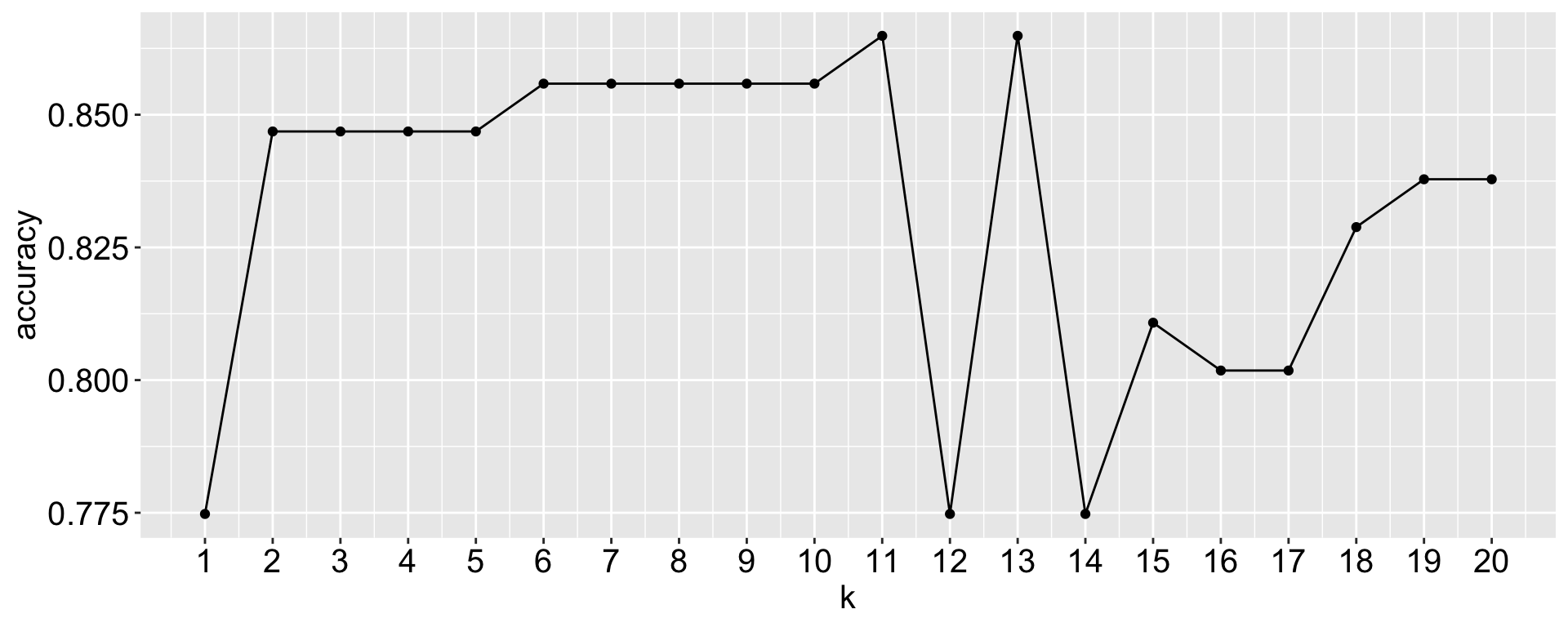
What would be the best k?

A naive try: for what we have done, run the kknn() for different k values and see which one gives the best accuracy on the testing set.

Here I compute the proportion of accurate prediction for each k from 1 to 20. Which k would you choose?

Does that mean k = 11/ 13 is the best k?

What would be the best k?

Not necessarily! Because the training-testing split is random, different splits may lead to different best k values.

• seed: 123, best k = 11 or 13
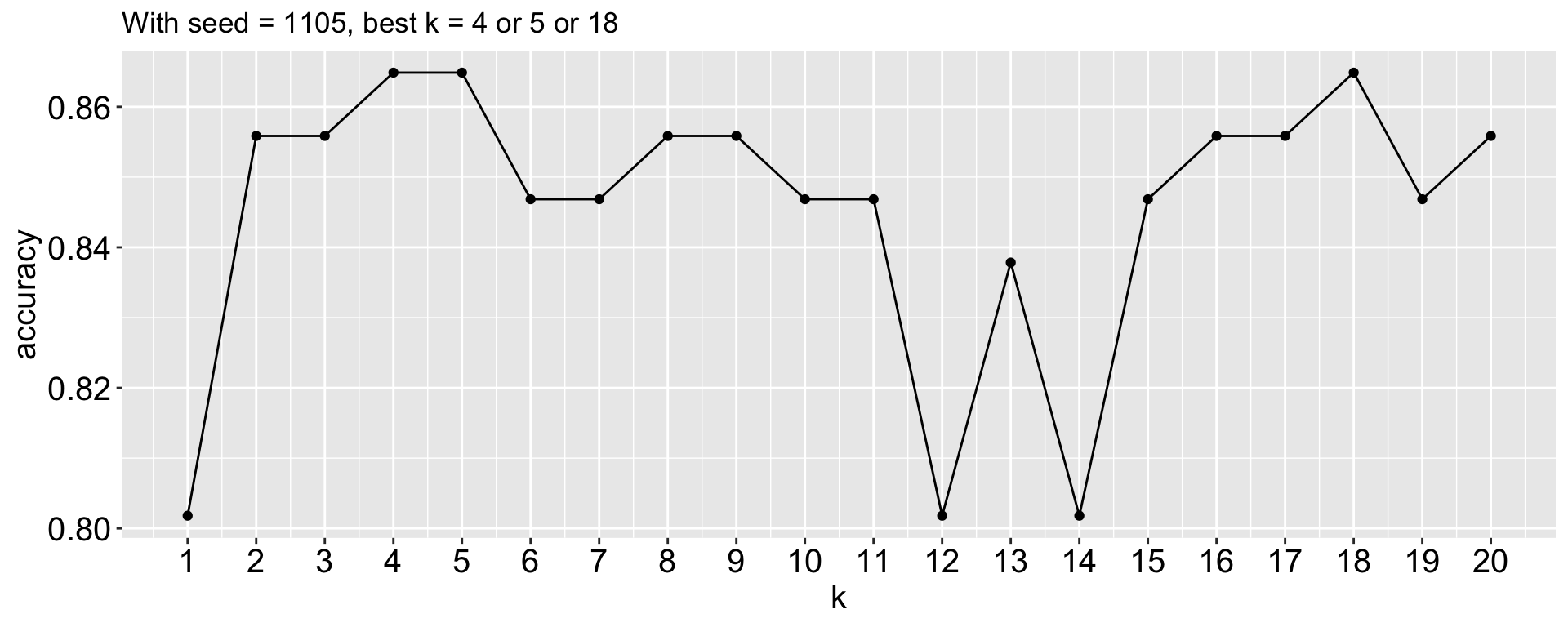
• seed: 12345, best k = 4 or 5 or 18
• seed: 1105, best k = 13

# Step 1: conduct the same training testing split
penguins_std <- penguins_clean |> 
  select(bill_len, bill_dep) |> 
  scale() |> 
  bind_cols(sex = penguins_clean2$sex)
m <- nrow(penguins_std)
set.seed(12345)
val <- sample(1:m, size = round(m/3), replace = FALSE)
penguins_training2 <- penguins_std[-val,]
penguins_testing2 <- penguins_std[val,]



# Step 2: fit the KNN model with different k_vec
# you can think of this as for each k, we make a prediction of the 111 testing points
# this gives us 20 * 111 = 2220 predictions
k_vec <- 1:20
k_res <- map_dfr(k_vec, function(k){
  knn_res2 <- kknn(sex ~ bill_len + bill_dep, k = k,
                   train = penguins_training2, test = penguins_testing2)
  res <- tibble(pred_class = predict(knn_res2))
  tibble(pred = res$pred_class, sex = penguins_testing2$sex)
}, .id = "k")

# Step 3: compute the prediction accuracy for each k and plot it
acc_count_df <- k_res |> 
  group_split(k) |> 
  map_dfr(~count(.x, pred, sex), .id = "k") |> 
  filter(pred == sex) |> 
  mutate(k = as.integer(k)) |> 
  group_by(k) |> 
  summarize(accuracy = sum(n) / 111) 

acc_count_df |>
  ggplot(aes(x = k, y = accuracy)) +
  geom_line() +
  geom_point() +
  scale_x_continuous(breaks = 1:20) + 
  ggtitle("With seed = 1105, best k = 4 or 5 or 18")

We have lot of variability in the best k depending on the training-testing split.

Cross validation

To reduce the variance, we would like some average performance across different training-testing splits - This is the idea behind cross validation.

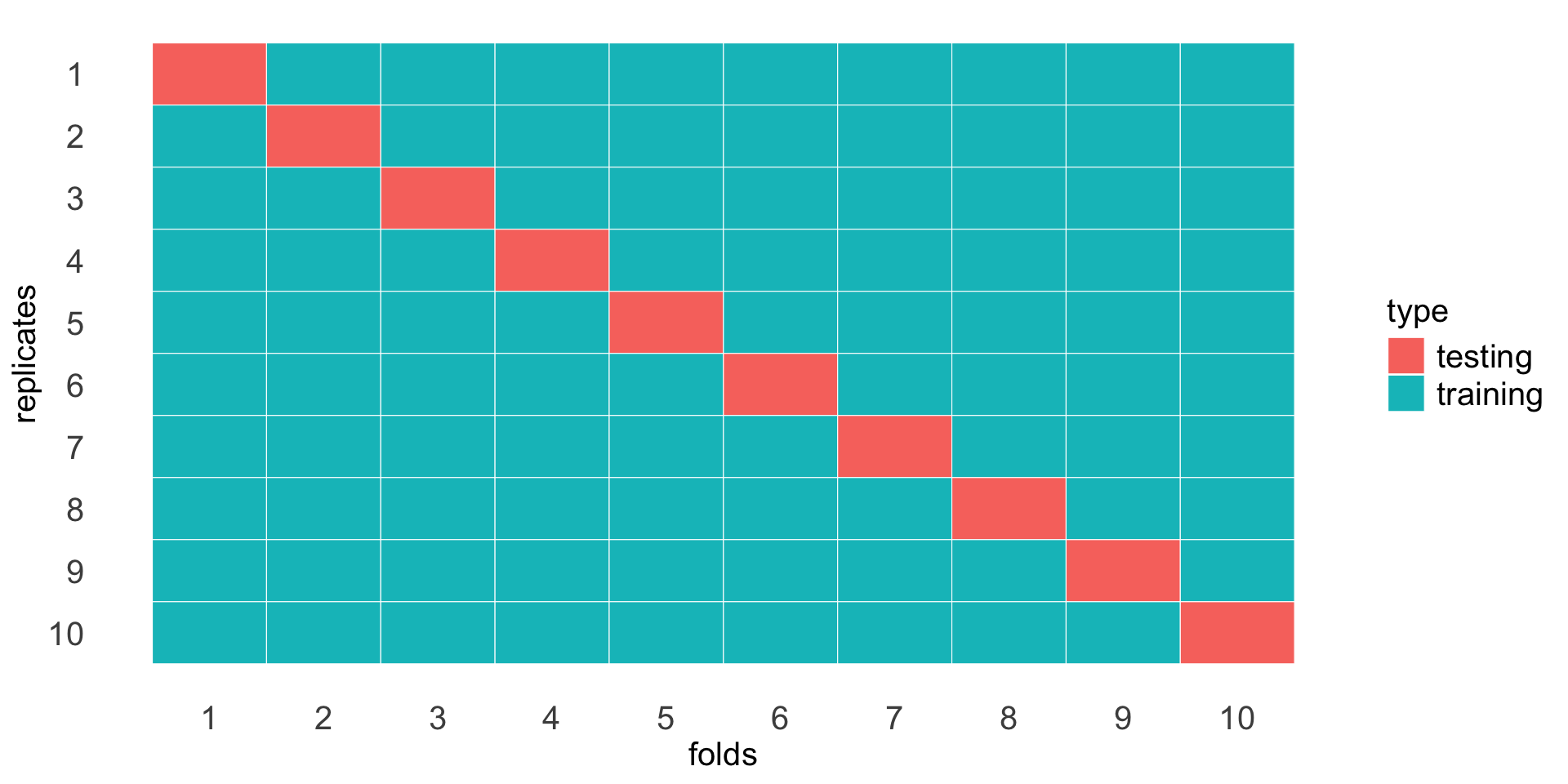
We can split the data into 10 folds (or any number of folds), and use 9 folds as training and 1 fold as testing, repeat this for each fold as testing, and average the accuracy across the 10 folds for each k.

A not so little script to do cross validation for KNN

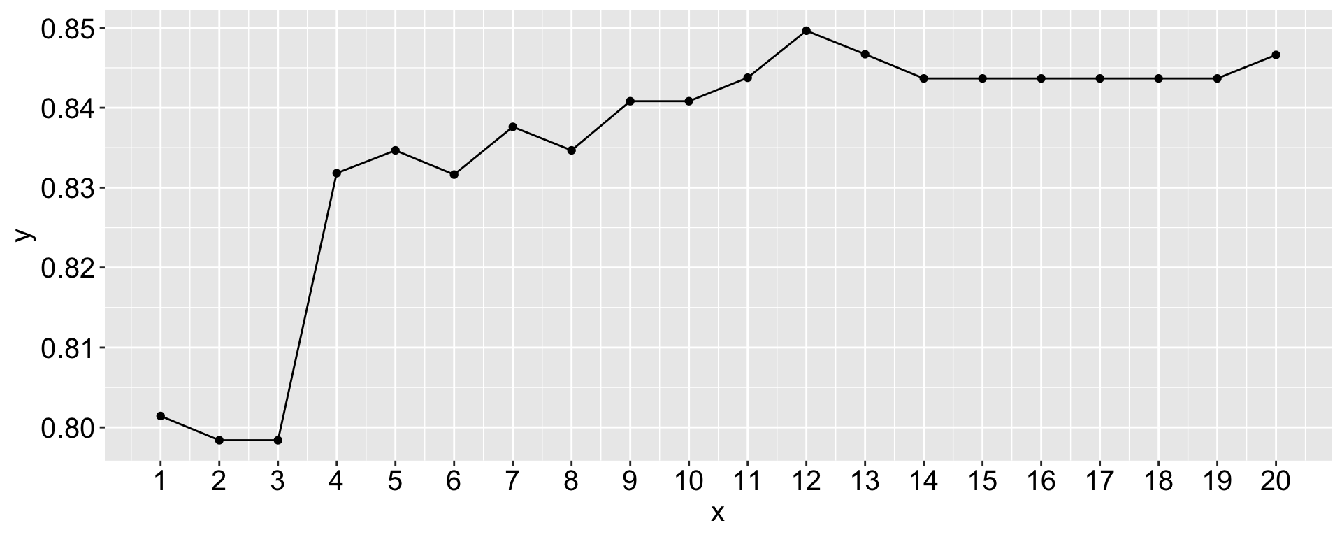
library(kknn)
library(caret)
set.seed(123)
penguins_clean <- as_tibble(datasets::penguins) |> na.omit() 

penguins_std <- penguins_clean |> 
  select(bill_len, bill_dep) |> 
  scale() |> 
  bind_cols(sex = penguins_clean$sex)


folds <- createFolds(penguins_std$sex, k = 10)

k_values <- 1:20
acc_k <- numeric(length(k_values))

for (j in seq_along(k_values)) {
  acc_fold <- c()
  
  for (i in 1:10) {
    test_idx <- folds[[i]]
    train_data <- penguins_std[-test_idx, ]
    test_data  <- penguins_std[test_idx, ]
    
    mod <- kknn(sex ~ bill_len + bill_dep,
                train = train_data,
                test = test_data,
                k = k_values[j])
    
    pred <- fitted(mod)
    acc_fold[i] <- mean(pred == test_data$sex)
  }
  
  acc_k[j] <- mean(acc_fold)
}

# Show best k
best_k <- k_values[which.max(acc_k)]
tibble(x = 1:20, y = acc_k) |> 
  ggplot(aes(x = x, y = y)) +
  geom_point() +
  geom_line() +
  scale_x_continuous(breaks = 1:20)

You’re not required to write this code! We will learn how to specify it with tidymodels in the next class.