# A tibble: 344 × 8
   species island    bill_len bill_dep flipper_len body_mass sex     year
   <fct>   <fct>        <dbl>    <dbl>       <int>     <int> <fct>  <int>
 1 Adelie  Torgersen     39.1     18.7         181      3750 male    2007
 2 Adelie  Torgersen     39.5     17.4         186      3800 female  2007
 3 Adelie  Torgersen     40.3     18           195      3250 female  2007
 4 Adelie  Torgersen     NA       NA            NA        NA <NA>    2007
 5 Adelie  Torgersen     36.7     19.3         193      3450 female  2007
 6 Adelie  Torgersen     39.3     20.6         190      3650 male    2007
 7 Adelie  Torgersen     38.9     17.8         181      3625 female  2007
 8 Adelie  Torgersen     39.2     19.6         195      4675 male    2007
 9 Adelie  Torgersen     34.1     18.1         193      3475 <NA>    2007
10 Adelie  Torgersen     42       20.2         190      4250 <NA>    2007
# ℹ 334 more rowsElements of Data Science
SDS 322E
H. Sherry Zhang
Department of Statistics and Data Sciences
The University of Texas at Austin
Fall 2025
Department of Statistics and Data Sciences
The University of Texas at Austin
Fall 2025
Learning objective
Understand the K-means clustering algorithm on a high level
Perform the K-means clustering using R
Cluster analysis in life
Imagine you’re a store manager at a supermarket, and you need to decide how to arrange these sport equipment into two shelves:
- dumbbell,
- barbell,
- swimsuit,
- golf club,
- tennis racket,
- resistant band
One solution:
- Group 1: gym equipment: dumbbell, barbell, resistant band.
- Group 2: outdoor sport equipment: swimsuit, golf club, tennis racket.
Cluster analysis
Clustering looks to group items (observations) into clusters that are similar within clusters and dissimilar between clusters.
In K-means clustering (today), we know the number of clusters we want to cluster the items into (2 clusters for sport equipment).
In hierarchical clustering (Friday), we do not know in advance how many clusters we want.
The K-means clustering algorithm
Artwork by @allison_horst
Artwork by @allison_horst
Artwork by @allison_horst
Artwork by @allison_horst
Artwork by @allison_horst
Artwork by @allison_horst
Artwork by @allison_horst
Artwork by @allison_horst
Artwork by @allison_horst
Artwork by @allison_horst
Artwork by @allison_horst
Kmeans clustering as an optimization problem
We can characterise the kmeans algorithm as an optimization problem that
minimize the within-cluster variation: squared Euclidean distance.
What you’ve just seen is an algorithm that can solve the optimisation.
However, this algorithm only finds the locally optimal solution, and the result depends on the initial random assignment of cluster labels. Recommend running the algorithm multiple times: the
nstartargument in thekmeans()function.
Choosing the number of clusters K
The kmeans algorithm requires the user to specify the number of clusters K in advance.
Based on domain knowledge
Elbow method: plot the total within-cluster variation against the number of clusters K, and look for an “elbow” in the plot.
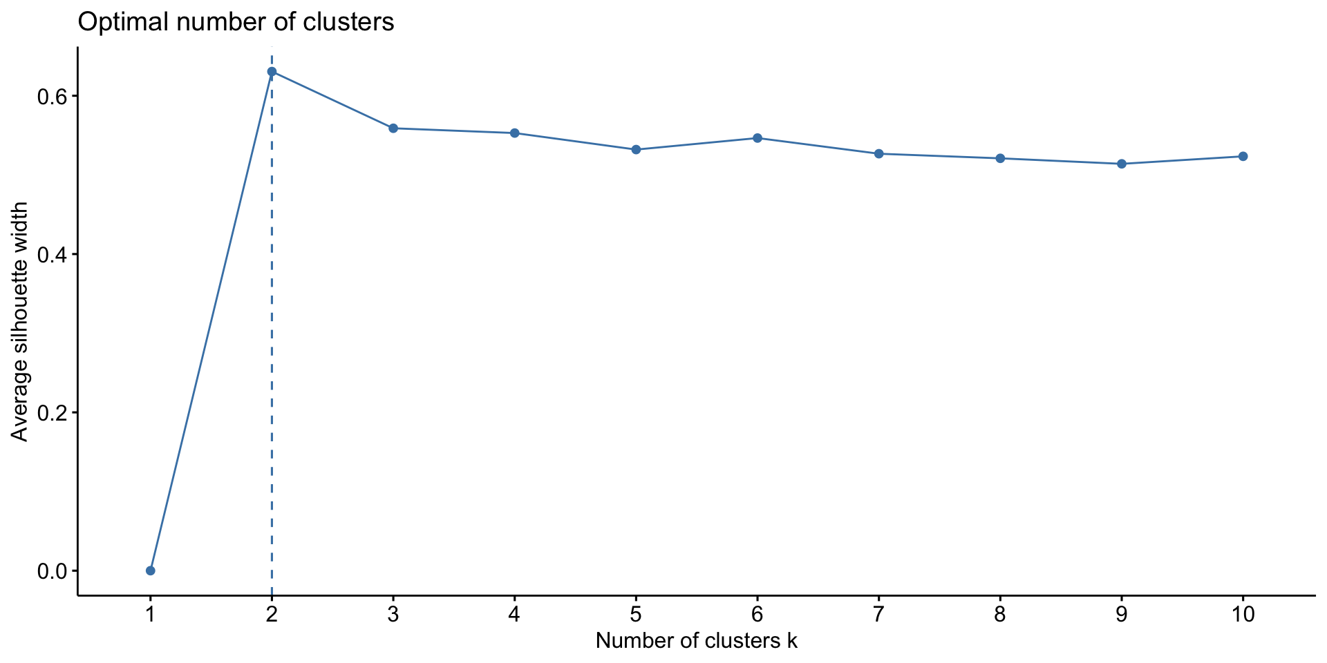
Silhouette method: measure how far each observation is from the observations in its own cluster compared to those in the nearest cluster. Average silhouette width can be computed for different values of K, and the value of K that maximizes the average silhouette width is chosen.
Gap statistic: compare the total within-cluster variation for different values of K with their expected values under a null reference distribution of the data. The value of K that maximizes the gap statistic is chosen.
Different methods may give different suggestions for the optimal number of clusters.
Use factoextra package to visualize the results of these methods: fviz_nbcluster(DATA, kmeans, method = "...") function.
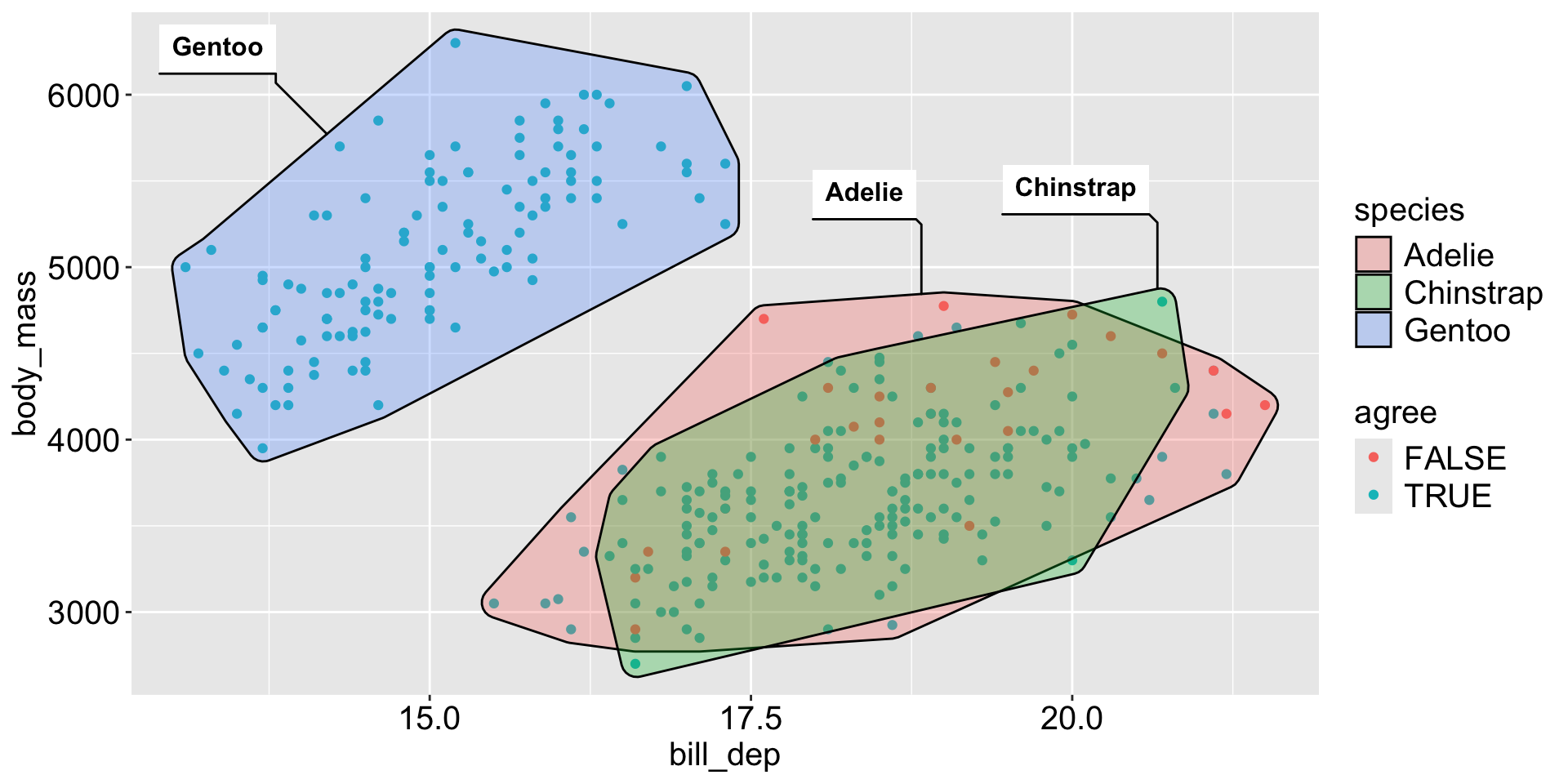
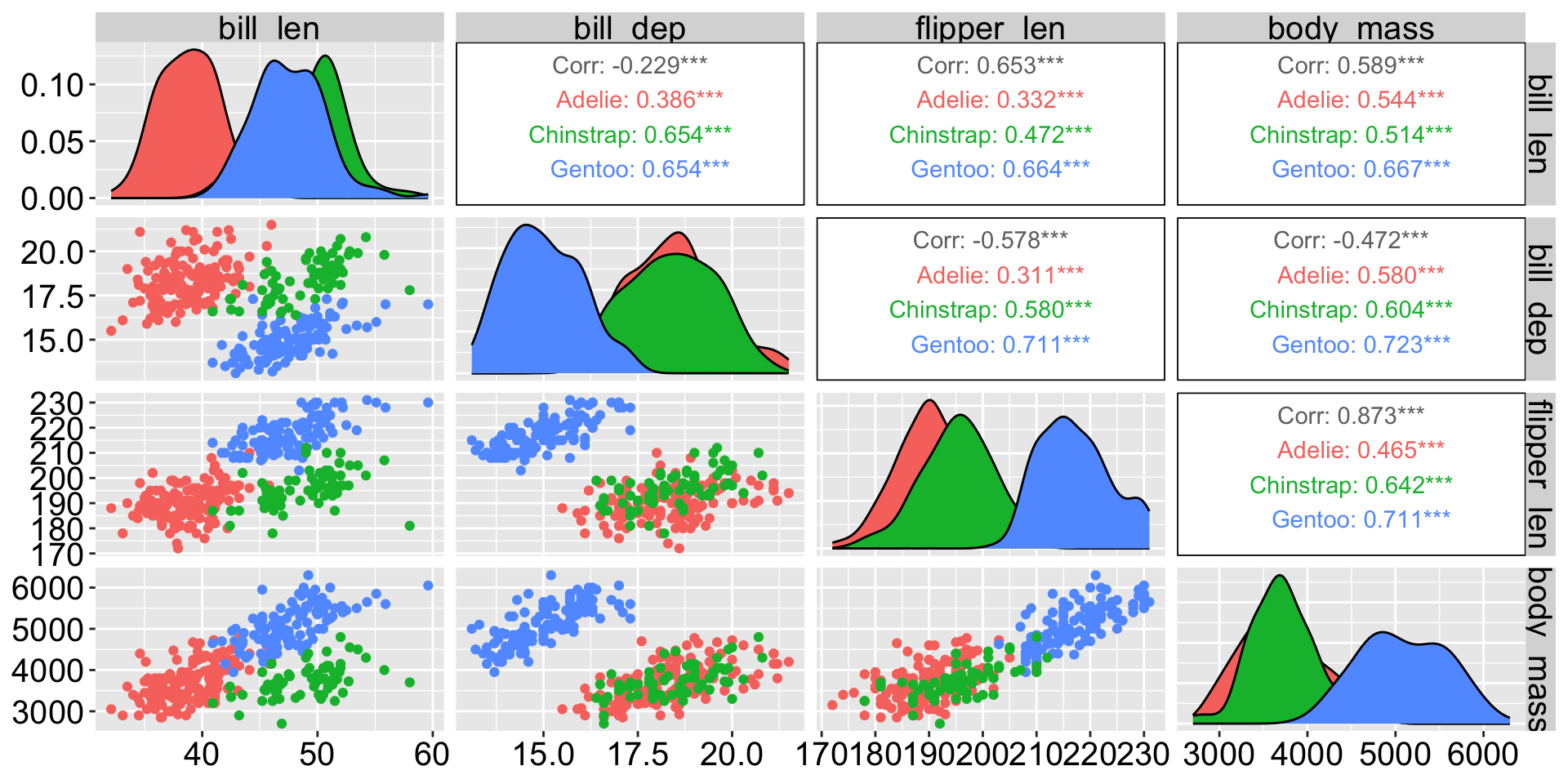
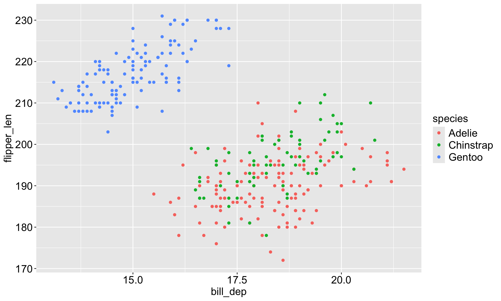
Example: Penguins data
Make sure you’re using the base R penguins dataset, not the one from palmerpenguins package.
Artwork by @allison_horst
Kmeans pre-processing
Follow along the class example with
usethis::create_from_github(""SDS322E-2025Fall/0902-kmeans")
Missing values are not allowed in kmeans. Why? . . .
# A tibble: 333 × 8
   species island    bill_len bill_dep flipper_len body_mass sex     year
   <fct>   <fct>        <dbl>    <dbl>       <int>     <int> <fct>  <int>
 1 Adelie  Torgersen     39.1     18.7         181      3750 male    2007
 2 Adelie  Torgersen     39.5     17.4         186      3800 female  2007
 3 Adelie  Torgersen     40.3     18           195      3250 female  2007
 4 Adelie  Torgersen     36.7     19.3         193      3450 female  2007
 5 Adelie  Torgersen     39.3     20.6         190      3650 male    2007
 6 Adelie  Torgersen     38.9     17.8         181      3625 female  2007
 7 Adelie  Torgersen     39.2     19.6         195      4675 male    2007
 8 Adelie  Torgersen     41.1     17.6         182      3200 female  2007
 9 Adelie  Torgersen     38.6     21.2         191      3800 male    2007
10 Adelie  Torgersen     34.6     21.1         198      4400 male    2007
# ℹ 323 more rows
Distance is going to be large for body_mass_g (in thousands) and bill_length_mm (in mm), while small for flipper_length_mm (in mm) - is this an issue?
Kmeans pre-processing
Yes! The base R scale() function does 2 things:
centers the variables to have mean 0 - this is optional for kmeans
scales the variables to have standard deviation 1 - we need this for kmeans
Think about why this is the case?
       bill_len  bill_dep flipper_len  body_mass
[1,] -0.8946955 0.7795590  -1.4246077 -0.5676206
[2,] -0.8215515 0.1194043  -1.0678666 -0.5055254
[3,] -0.6752636 0.4240910  -0.4257325 -1.1885721
[4,] -1.3335592 1.0842457  -0.5684290 -0.9401915
[5,] -0.8581235 1.7444004  -0.7824736 -0.6918109
[6,] -0.9312674 0.3225288  -1.4246077 -0.7228585
Kmeans: choose the number of clusters K
Kmeans: choose the number of clusters K
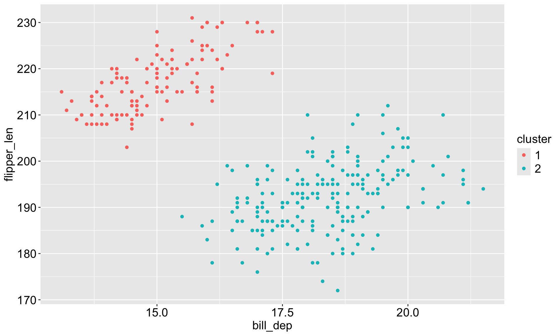
Kmeans results
The base R function kmeans() performs kmeans clustering.
Use set.seed() so that the initial cluster assignments can be replicated.
K-means clustering with 2 clusters of sizes 119, 214

Cluster means:
    bill_len  bill_dep flipper_len  body_mass
1  0.6537742 -1.101050    1.160716  1.0995561
2 -0.3635474  0.612266   -0.645445 -0.6114354

Clustering vector:
  [1] 2 2 2 2 2 2 2 2 2 2 2 2 2 2 2 2 2 2 2 2 2 2 2 2 2 2 2 2 2 2 2 2 2 2 2 2 2
 [38] 2 2 2 2 2 2 2 2 2 2 2 2 2 2 2 2 2 2 2 2 2 2 2 2 2 2 2 2 2 2 2 2 2 2 2 2 2
 [75] 2 2 2 2 2 2 2 2 2 2 2 2 2 2 2 2 2 2 2 2 2 2 2 2 2 2 2 2 2 2 2 2 2 2 2 2 2
[112] 2 2 2 2 2 2 2 2 2 2 2 2 2 2 2 2 2 2 2 2 2 2 2 2 2 2 2 2 2 2 2 2 2 2 2 1 1
[149] 1 1 1 1 1 1 1 1 1 1 1 1 1 1 1 1 1 1 1 1 1 1 1 1 1 1 1 1 1 1 1 1 1 1 1 1 1
[186] 1 1 1 1 1 1 1 1 1 1 1 1 1 1 1 1 1 1 1 1 1 1 1 1 1 1 1 1 1 1 1 1 1 1 1 1 1
[223] 1 1 1 1 1 1 1 1 1 1 1 1 1 1 1 1 1 1 1 1 1 1 1 1 1 1 1 1 1 1 1 1 1 1 1 1 1
[260] 1 1 1 1 1 1 2 2 2 2 2 2 2 2 2 2 2 2 2 2 2 2 2 2 2 2 2 2 2 2 2 2 2 2 2 2 2
[297] 2 2 2 2 2 2 2 2 2 2 2 2 2 2 2 2 2 2 2 2 2 2 2 2 2 2 2 2 2 2 2 2 2 2 2 2 2

Within cluster sum of squares by cluster:
[1] 139.4684 411.5430
 (between_SS / total_SS =  58.5 %)

Available components:

[1] "cluster"      "centers"      "totss"        "withinss"     "tot.withinss"
[6] "betweenss"    "size"         "iter"         "ifault"
Kmeans results
The kmeans_results object is a list with several components. Use $ to access each component, e.g. kmeans_results$centers gives the cluster centers.
  [1] 2 2 2 2 2 2 2 2 2 2 2 2 2 2 2 2 2 2 2 2 2 2 2 2 2 2 2 2 2 2 2 2 2 2 2 2 2
 [38] 2 2 2 2 2 2 2 2 2 2 2 2 2 2 2 2 2 2 2 2 2 2 2 2 2 2 2 2 2 2 2 2 2 2 2 2 2
 [75] 2 2 2 2 2 2 2 2 2 2 2 2 2 2 2 2 2 2 2 2 2 2 2 2 2 2 2 2 2 2 2 2 2 2 2 2 2
[112] 2 2 2 2 2 2 2 2 2 2 2 2 2 2 2 2 2 2 2 2 2 2 2 2 2 2 2 2 2 2 2 2 2 2 2 1 1
[149] 1 1 1 1 1 1 1 1 1 1 1 1 1 1 1 1 1 1 1 1 1 1 1 1 1 1 1 1 1 1 1 1 1 1 1 1 1
[186] 1 1 1 1 1 1 1 1 1 1 1 1 1 1 1 1 1 1 1 1 1 1 1 1 1 1 1 1 1 1 1 1 1 1 1 1 1
[223] 1 1 1 1 1 1 1 1 1 1 1 1 1 1 1 1 1 1 1 1 1 1 1 1 1 1 1 1 1 1 1 1 1 1 1 1 1
[260] 1 1 1 1 1 1 2 2 2 2 2 2 2 2 2 2 2 2 2 2 2 2 2 2 2 2 2 2 2 2 2 2 2 2 2 2 2
[297] 2 2 2 2 2 2 2 2 2 2 2 2 2 2 2 2 2 2 2 2 2 2 2 2 2 2 2 2 2 2 2 2 2 2 2 2 2
kmean_df <- penguins_clean |> bind_cols(tibble(cluster = as.factor(kmeans_results$cluster)))
kmean_df# A tibble: 333 × 9
species island bill_len bill_dep flipper_len body_mass sex year cluster
<fct> <fct> <dbl> <dbl> <int> <int> <fct> <int> <fct>
1 Adelie Torgersen 39.1 18.7 181 3750 male 2007 2
2 Adelie Torgersen 39.5 17.4 186 3800 fema… 2007 2
3 Adelie Torgersen 40.3 18 195 3250 fema… 2007 2
4 Adelie Torgersen 36.7 19.3 193 3450 fema… 2007 2
5 Adelie Torgersen 39.3 20.6 190 3650 male 2007 2
6 Adelie Torgersen 38.9 17.8 181 3625 fema… 2007 2
7 Adelie Torgersen 39.2 19.6 195 4675 male 2007 2
8 Adelie Torgersen 41.1 17.6 182 3200 fema… 2007 2
9 Adelie Torgersen 38.6 21.2 191 3800 male 2007 2
10 Adelie Torgersen 34.6 21.1 198 4400 male 2007 2
# ℹ 323 more rowsKmeans results visualization
What about we choose K = 3?
set.seed(123)
res <- kmeans_df |>
  kmeans(centers = 3, nstart = 20)

# look at how the clusters align with species
penguins_clean |>
  bind_cols(tibble(cluster = as.factor(res$cluster))) |>
  count(species, cluster)
# A tibble: 5 × 3
species cluster n
<fct> <fct> <int>
1 Adelie 1 22
2 Adelie 2 124
3 Chinstrap 1 63
4 Chinstrap 2 5
5 Gentoo 3 119