# A tibble: 344 × 8
   species island    bill_len bill_dep flipper_len body_mass sex     year
   <fct>   <fct>        <dbl>    <dbl>       <int>     <int> <fct>  <int>
 1 Adelie  Torgersen     39.1     18.7         181      3750 male    2007
 2 Adelie  Torgersen     39.5     17.4         186      3800 female  2007
 3 Adelie  Torgersen     40.3     18           195      3250 female  2007
 4 Adelie  Torgersen     NA       NA            NA        NA <NA>    2007
 5 Adelie  Torgersen     36.7     19.3         193      3450 female  2007
 6 Adelie  Torgersen     39.3     20.6         190      3650 male    2007
 7 Adelie  Torgersen     38.9     17.8         181      3625 female  2007
 8 Adelie  Torgersen     39.2     19.6         195      4675 male    2007
 9 Adelie  Torgersen     34.1     18.1         193      3475 <NA>    2007
10 Adelie  Torgersen     42       20.2         190      4250 <NA>    2007
# ℹ 334 more rowsElements of Data Science
SDS 322E
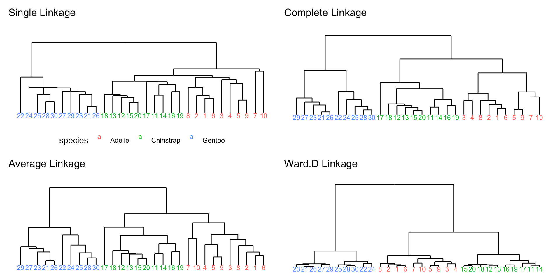
Visualize hierarchical clustering results
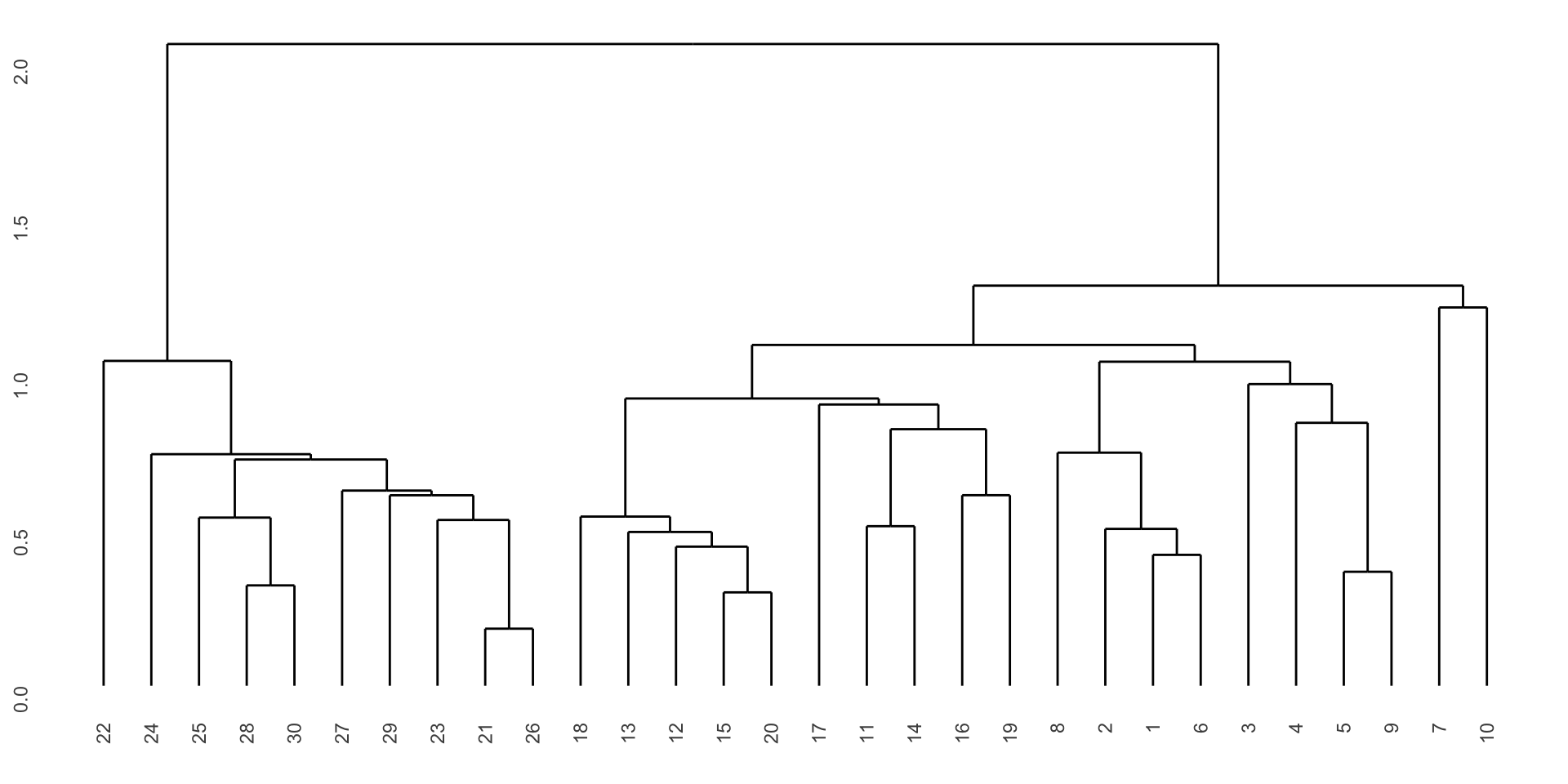
Visualize hierarchical clustering results
Code
hclust_data1 <- ggdendro::dendro_data(hclust_results1)
hclust_segments1 <- as_tibble(hclust_data1$segments)
hclust_labels1 <- as_tibble(hclust_data1$labels) |>
  mutate(species = penguins_small$species[as.integer(label)])

p1 <- ggplot() +
  geom_segment(data = hclust_segments1,
               aes(x = x, y = y, xend = xend, yend = yend)) +
  geom_text(data = hclust_labels1,
            aes(x = x, y = y - 0.02, label = label,
                color = species), vjust = 1, size = 3) +
  labs(title = "Single Linkage") +
  theme_minimal() +
  theme(axis.title = element_blank(),
        axis.text = element_blank(),
        axis.ticks = element_blank(),
        panel.grid = element_blank(),
        legend.position = "bottom") +
  ylim(-0.1, 2.5)
p1
Different linkage for penguins data
Full penguins data
Code
hclust_data <- ggdendro::dendro_data(hclust_results)
hclust_segments <- as_tibble(hclust_data$segments)
hclust_labels <- as_tibble(hclust_data$labels) |>
  mutate(species = penguins_clean$species[as.integer(label)])

ggplot() +
  geom_segment(data = hclust_segments,
               aes(x = x, y = y, xend = xend, yend = yend)) +
  geom_text(data = hclust_labels,
            aes(x = x, y = y - 0.02, label = label,
                color = species), vjust = 1, size = 3) +
  labs(title = "Average Linkage") +
  theme_minimal() +
  theme(axis.title = element_blank(),
        axis.text = element_blank(),
        axis.ticks = element_blank(),
        panel.grid = element_blank(),
        legend.position = "none") +
ylim(-0.1, 4) 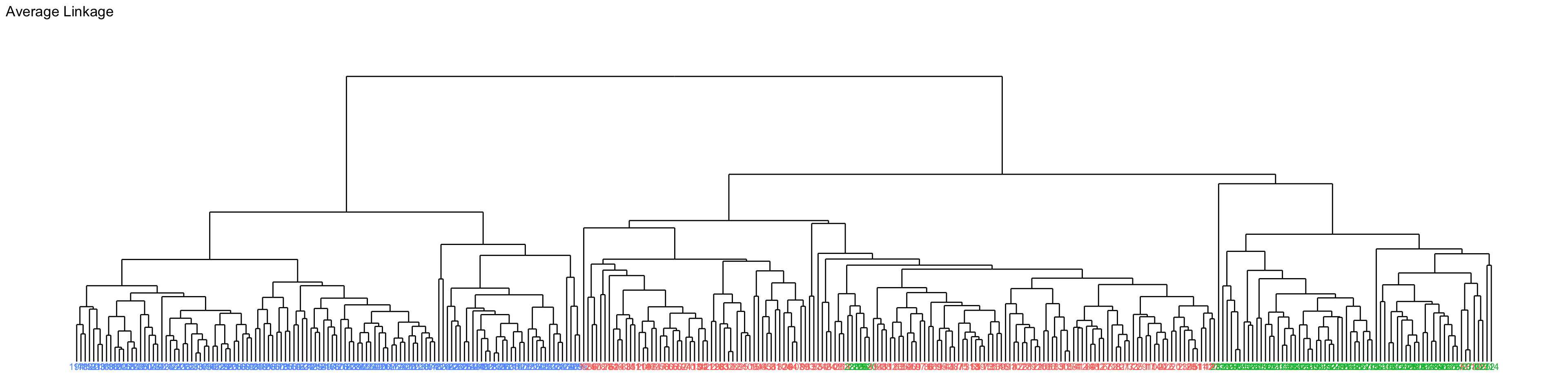
Cut the tree into two clusters
The base R function cutree() can be used to cut the dendrogram into a specified number of clusters.
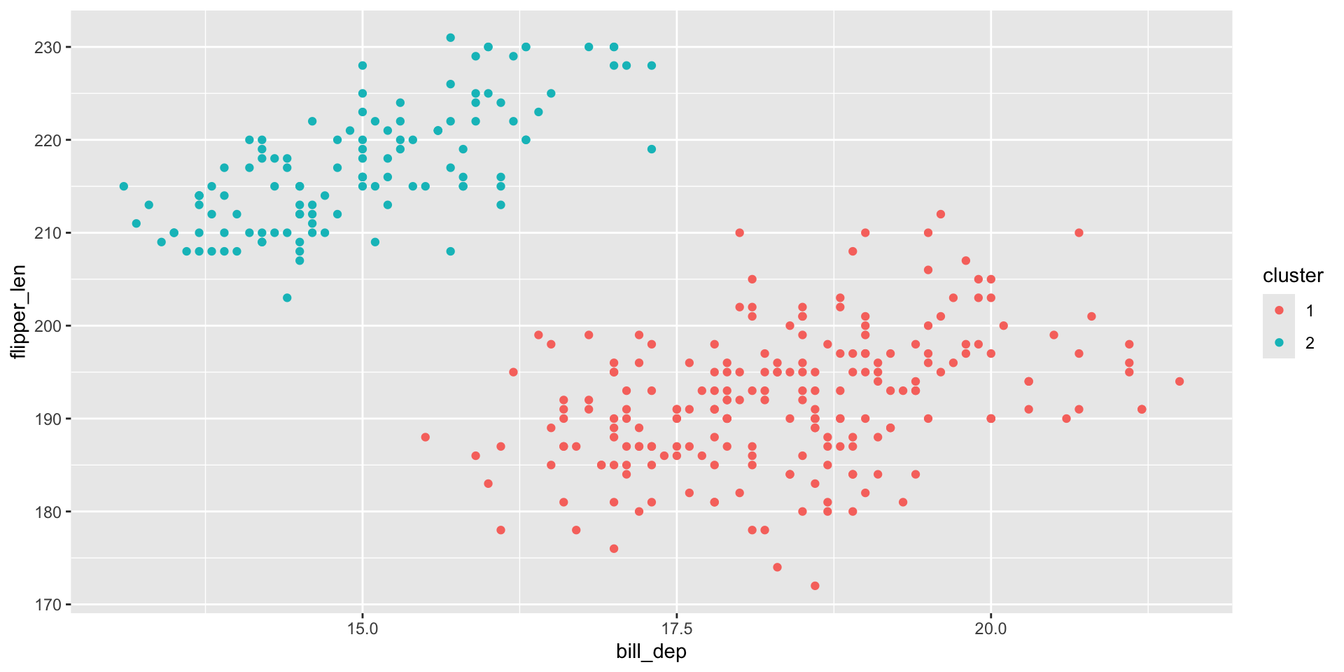
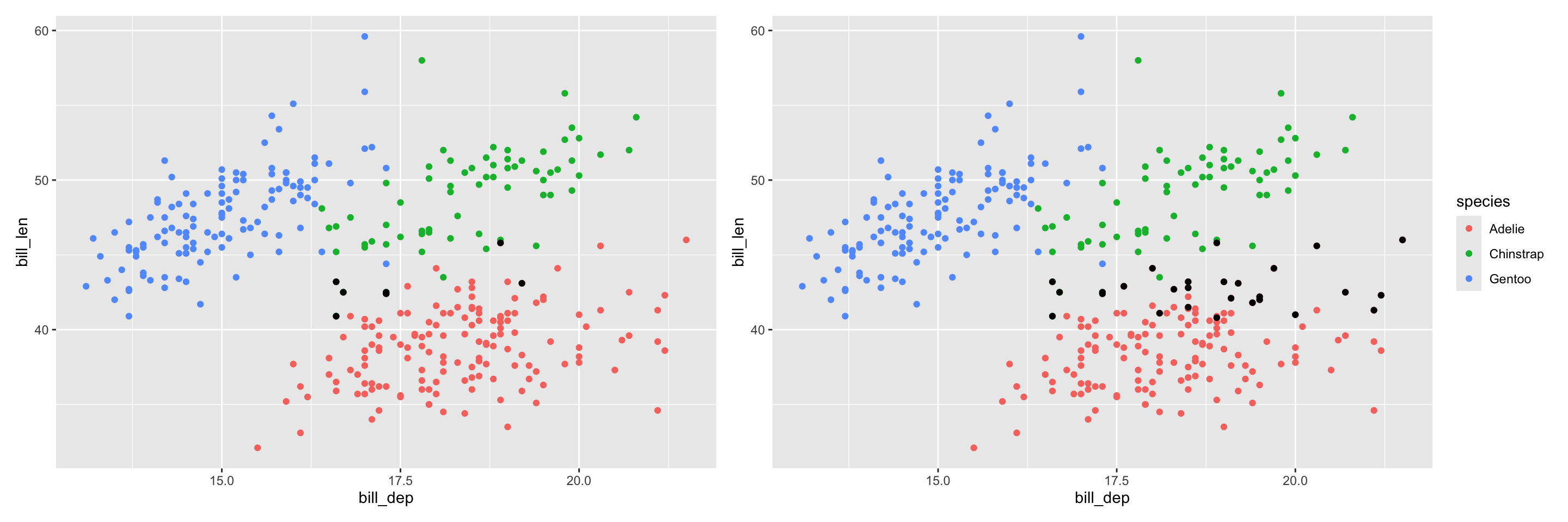
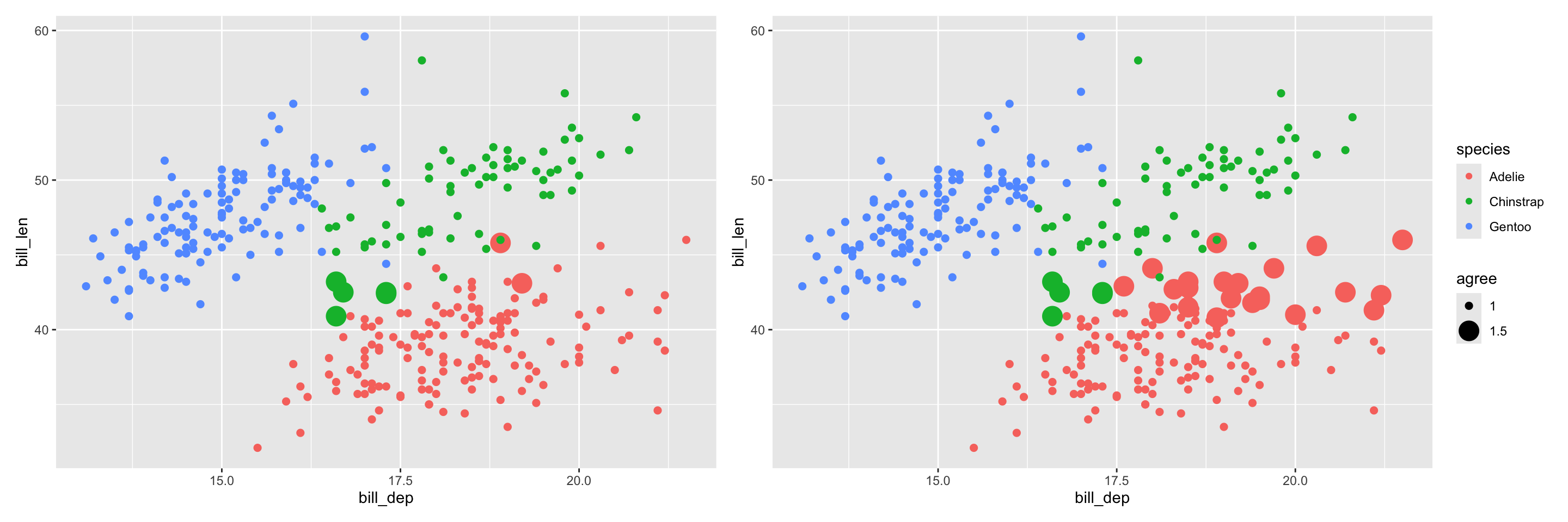
Compare hierarchical clustering with kmeans
Hierarchical clustering: cut into 3 groups
# A tibble: 5 × 3
  cluster species       n
  <fct>   <fct>     <int>
1 1       Adelie      144
2 1       Chinstrap     5
3 2       Adelie        2
4 2       Chinstrap    63
5 3       Gentoo      119
Kmeans clustering: choose 3 centers
# A tibble: 5 × 3
  cluster species       n
  <fct>   <fct>     <int>
1 1       Adelie      124
2 1       Chinstrap     5
3 2       Adelie       22
4 2       Chinstrap    63
5 3       Gentoo      119