All three models use the samepenguins_folds: each model is validated on exactly the same penguins, so their cross-validation results can be compared directly
strata = sex again: every fold keeps the same proportion of females and males
fit_resamples() (new): like tune_grid(), but for a model with nothing to tune: it fits the workflow on each fold and computes the validation metrics
save_pred = TRUE: keep the predictions on each validation fold, so we can draw ROC curves later
How many models? Logistic regression: 10 fits. KNN: 30 \(\times\) 10 = 300 fits. Random forest: 8 \(\times\) 10 = 80 forests of 500 trees, the slowest to tune
# A tibble: 3 × 4
  model                mean std_err     n
  <chr>               <dbl>   <dbl> <int>
1 Logistic regression 0.773  0.0292    10
2 KNN                 0.852  0.0221    10
3 Random forest       0.828  0.0292    10
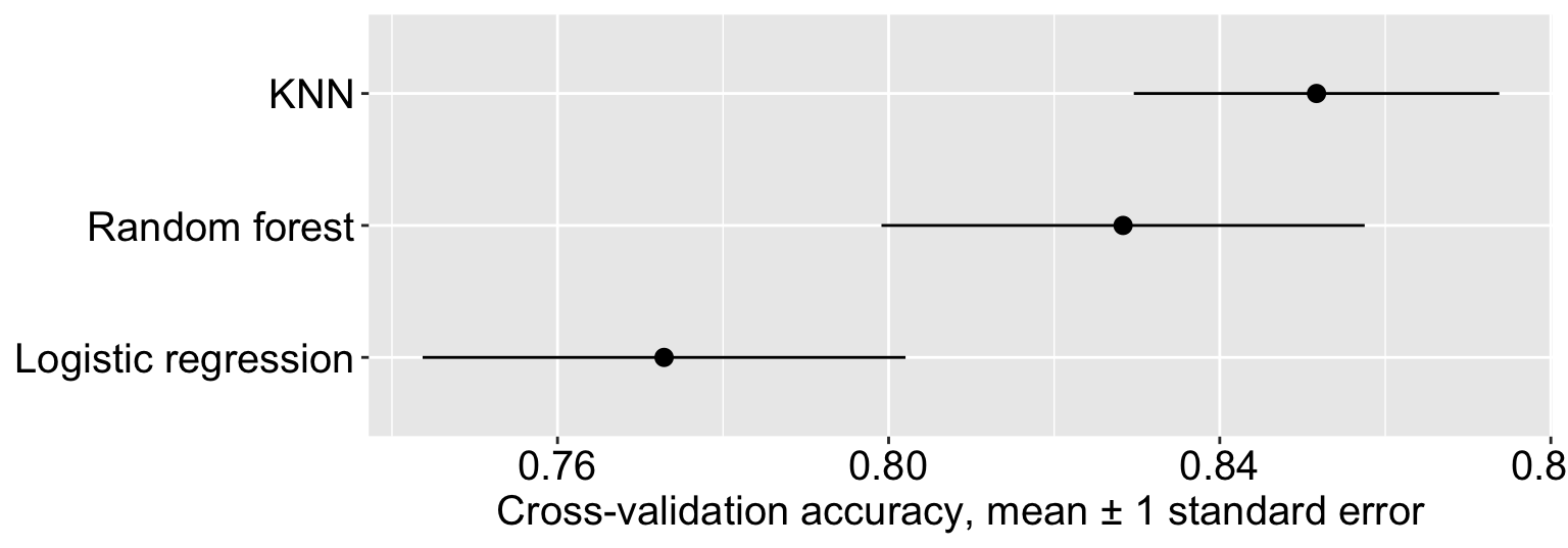
Plot the cross-validation accuracy with one standard error
cv_compare |>ggplot(aes(x = mean, y =fct_reorder(model, mean))) +geom_pointrange(aes(xmin = mean - std_err, xmax = mean + std_err)) +labs(x ="Cross-validation accuracy, mean ± 1 standard error", y =NULL)
Step 4.5: compare the ROC curves
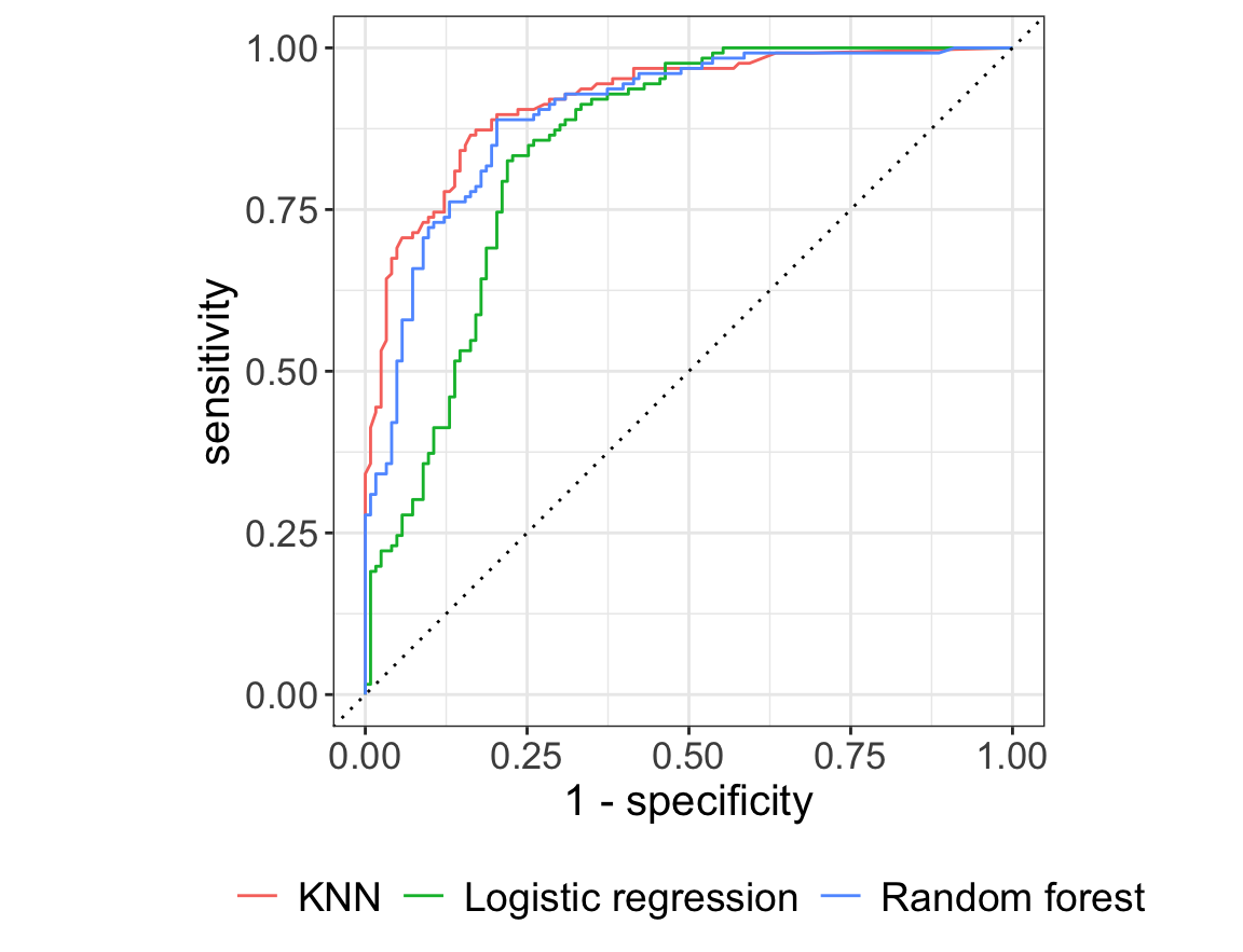
Accuracy depends on the 0.5 cutoff. The ROC curve compares the models over all cutoffs, using the predictions on the validation folds:
The closer a curve gets to the top-left corner, the better the model separates females and males (male = positive class)
The same conclusion as accuracy: KNN \(\approx\) random forest, both clearly better than logistic regression
Why does logistic regression lose?
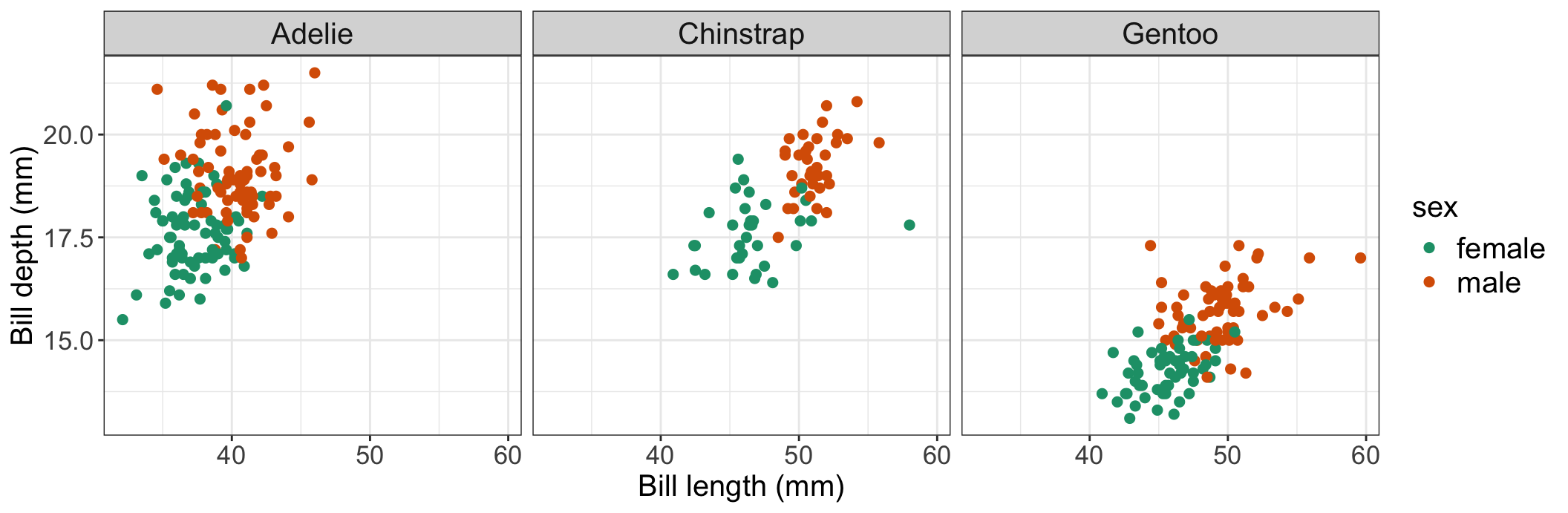
Within each species, males have bigger bills. But the species differ so much that a male Adelie and a female Chinstrap can have similar bills
So the boundary between female and male is not one straight line: it is in a different place for each species. Logistic regression can only draw one straight line; KNN and random forest can draw a flexible boundary
Step 5/6: evaluate the chosen model once
Plug the best \(k\) into the KNN workflow, refit on all the training data, and evaluate once on the testing data. last_fit() does the refit and the evaluation in one step:
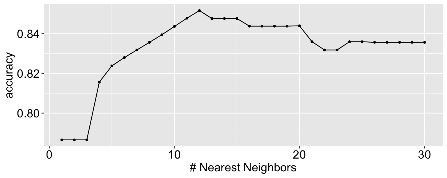
This is the number to report: how well the chosen model, KNN with \(k\) = 12, predicts new penguins
What about a regression problem?
If your response is numeric (e.g. predict body_mass), the same steps apply, with a few changes:
Models: linear_reg() instead of logistic_reg(), and mode = "regression" for KNN and random forest
Split: strata is optional: for a numeric response, strata = body_mass splits it into bins so every fold covers light and heavy penguins
Metrics: RMSE (in the units of the response) and \(R^2\), with metric_set(rmse, rsq): for RMSE, lower is better. Use select_best(metric = "rmse")
Recipes: the same rules. Dummy variables for categorical predictors in linear regression and KNN, normalization for KNN, nothing for the random forest
Don’t assume the flexible model wins: if the response is close to a straight-line function of the predictors (as body mass is of flipper length), linear regression can do as well as KNN and random forest, and is much easier to explain. Compare, and let the cross-validation results decide
For Project 2
Use this lecture as a template:
The question: what is one row, what is the response, and which predictors (no leakage!)?
Step 0: one training-testing split and one set of folds, shared by all models
Steps 1-4, for each model: a model, a recipe that suits it, a workflow, and cross-validation
Step 4.5: compare the models on the cross-validation metric, with its standard error: are the differences big enough to matter? Then choose a model, and explain why (performance, simplicity, interpretability)
Step 5/6: evaluate the chosen model once on the testing data, and report that number