Elements of Data Science
H. Sherry Zhang
Learning objectives
Understand the basic idea of decision trees for regression and classification
Fit decision trees using tidymodels for both regression and classification tasks
Identify the key parameters of decision trees and their effects
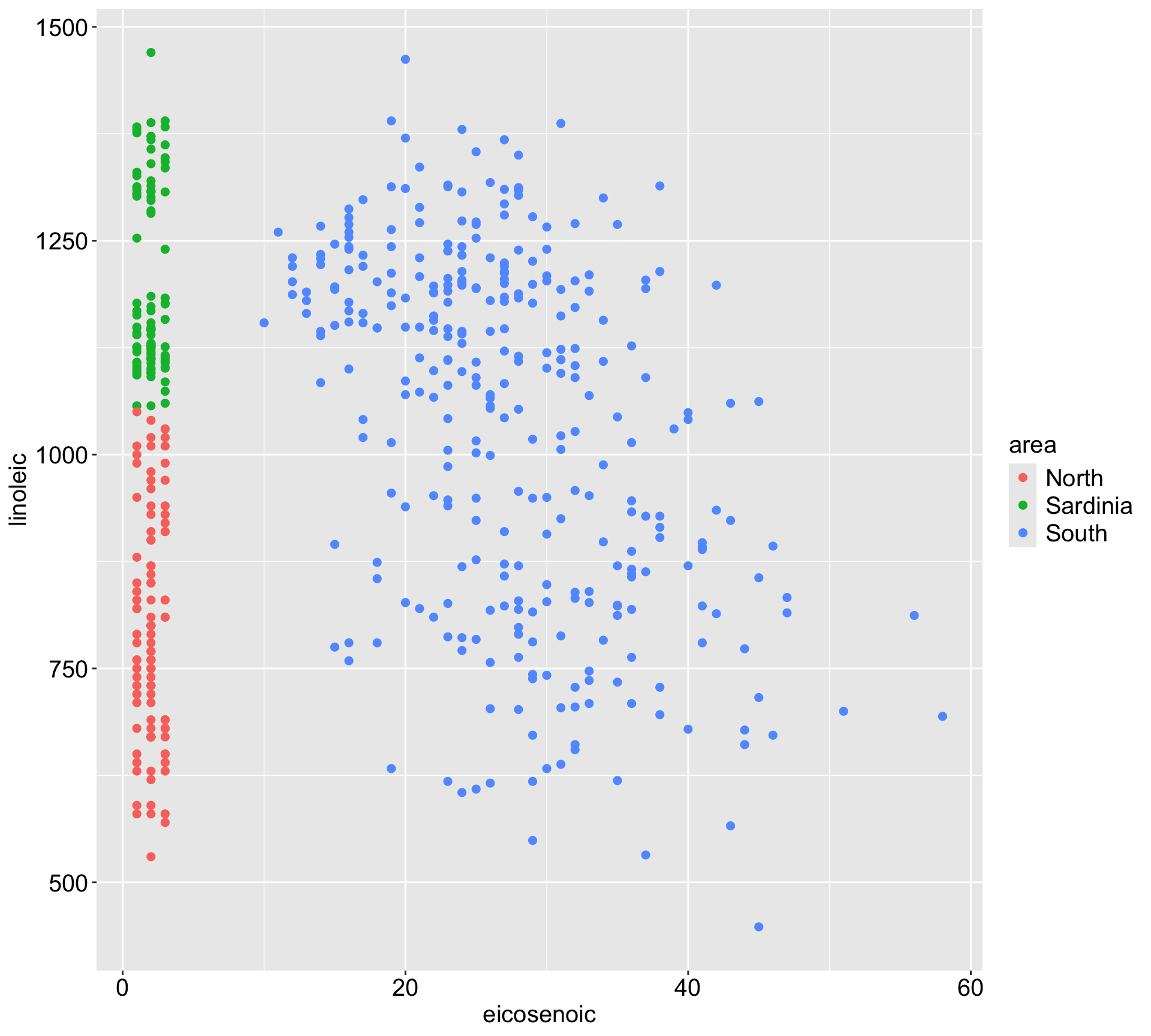
If we would like to predict the area from x1 (eicosenoic) and x2 (linoleic), would you expect linear regression or KNN to perform well?
Regression tree
Divide/partition the predictor space \(X_1, \ldots, X_p\) into \(J\) regions \(R_1, \ldots, R_J\) .
For every observation that falls within region \(R_j\) , we make the same prediction \(\bar{y}_{R_j}\) , which is the mean of the response values for the training observations in \(R_j\) .
For regression, the overall goal is typically to minimize the residual sum of squares:\[
RSS = \sum_{j=1}^{J} \sum_{i \in R_j} (y_i - \bar{y}_{R_j})^2\]
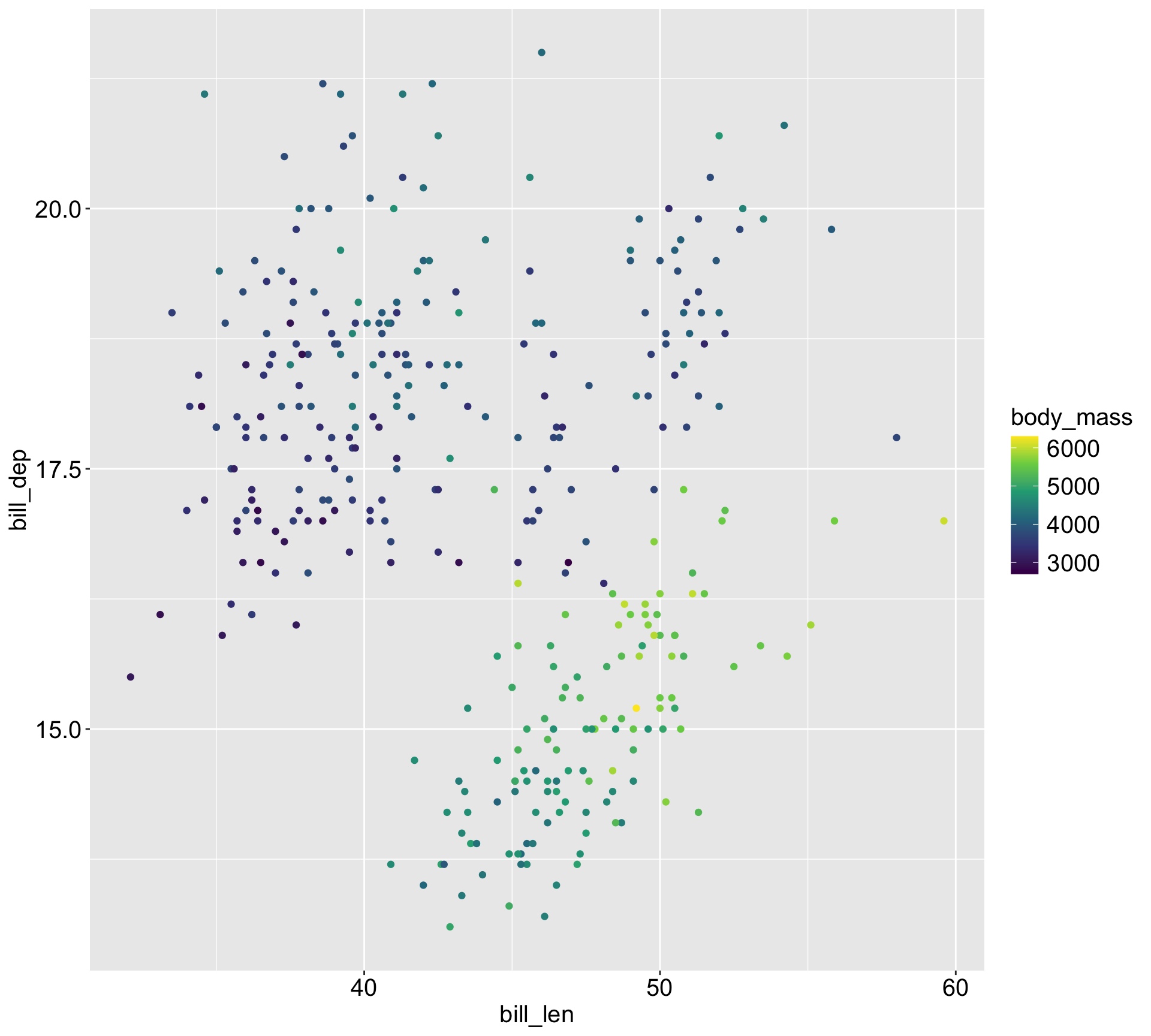
Regression tree with tidymodels Step 1/2/3: specify the model/ recipe/ workflow:
<- decision_tree (mode = "regression" , engine = "rpart" , min_n = 150 )<- recipe (body_mass ~ bill_len + bill_dep, data = datasets:: penguins) |> step_naomit ()<- workflow () |> add_model (dt_reg_spec) |> add_recipe (dt_recipe)
Step 4: fit the tree:
set.seed (1 )<- dt_wf |> fit (data = datasets:: penguins)
Step 5/6: predict/ calculate the prediction accuracy metrics:
|> augment (datasets:: penguins) |> metrics (truth = body_mass, estimate = .pred)
# A tibble: 3 × 3
  .metric .estimator .estimate
  <chr>   <chr>          <dbl>
1 rmse    standard     560.
2 rsq     standard       0.511
3 mae     standard     416.
Regression tree with tidymodels
|> extract_fit_engine ()
n=342 (2 observations deleted due to missingness)

node), split, n, deviance, yval
      * denotes terminal node

1) root 342 219307700 4201.754
  2) bill_dep>=16.45 220  65255400 3794.318
    4) bill_len< 39.05 76   9524836 3505.921 *
    5) bill_len>=39.05 144  46073260 3946.528 *
  3) bill_dep< 16.45 122  51673930 4936.475 *
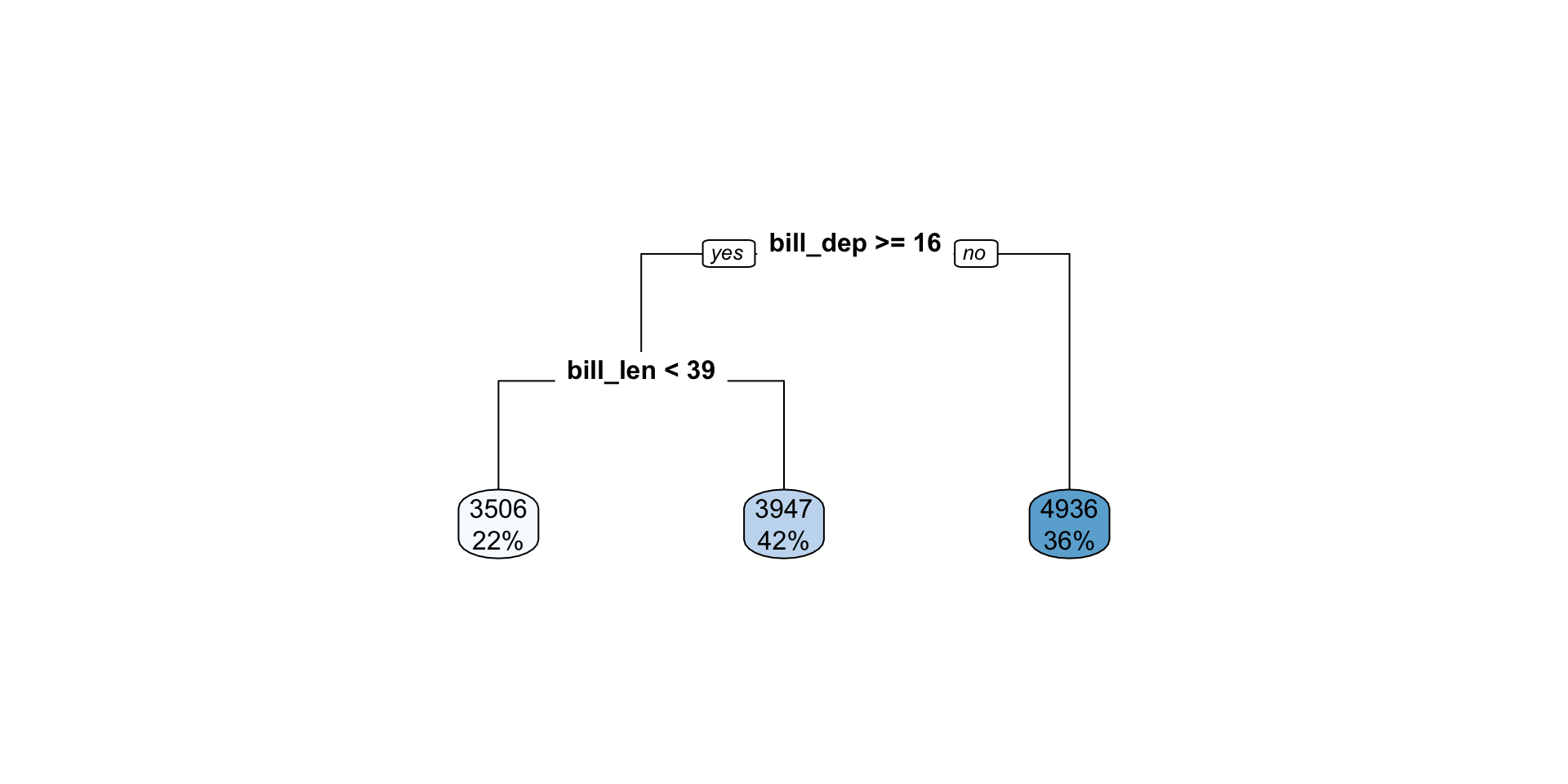
library (rpart.plot)|> extract_fit_engine () |> :: rpart.plot (type = 0 )
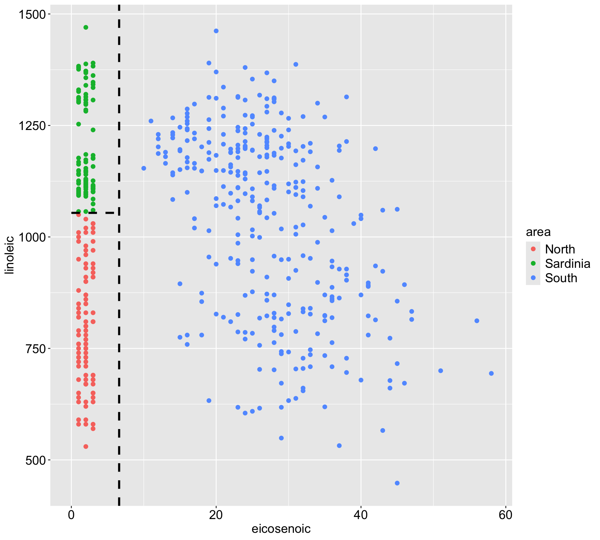
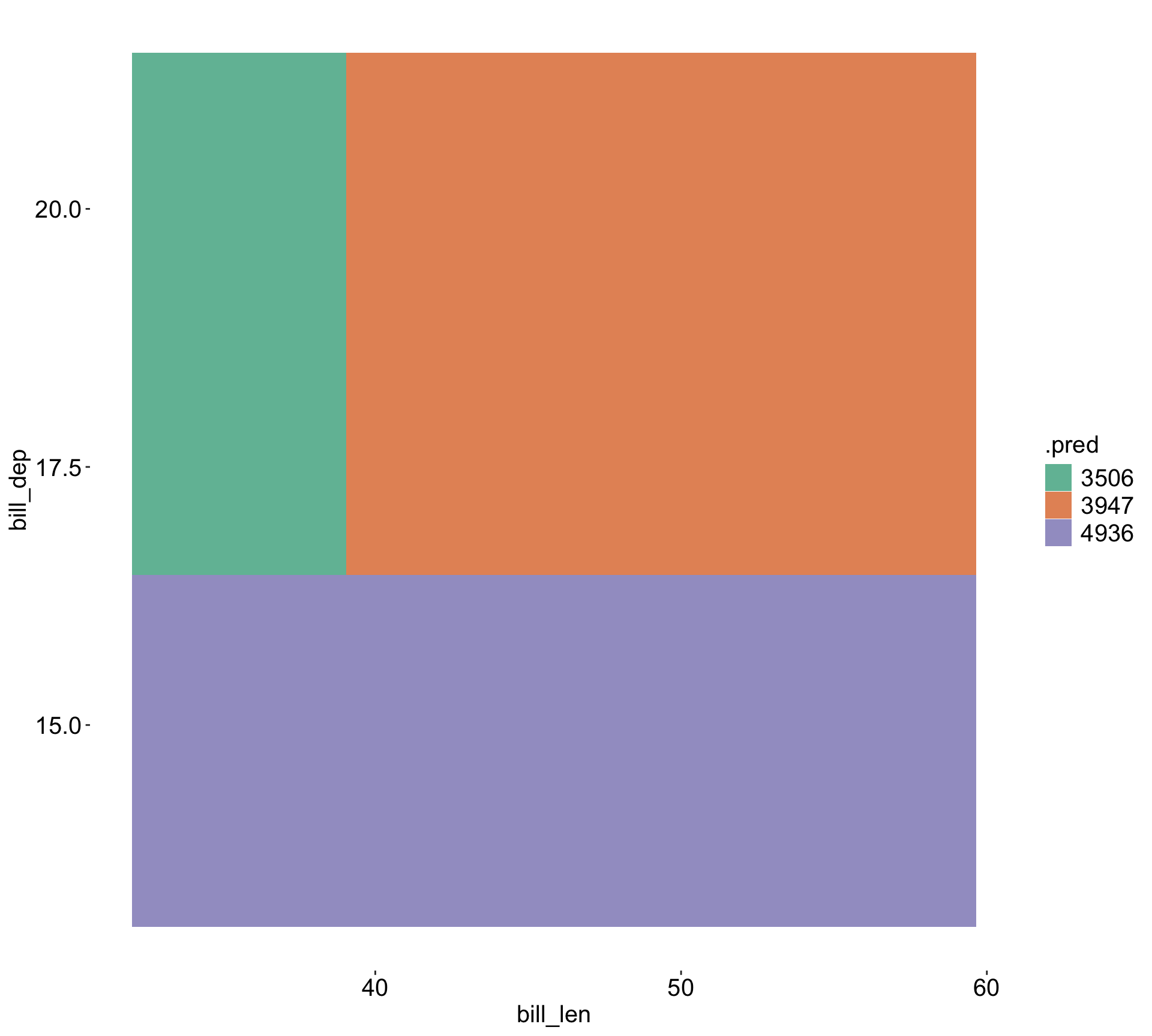
Visualize the space
Average body mass
3701
3733
5076
Classification tree
Classification trees use the same splits, but minimize impurity (not RSS).
Classification of an observation is taken as the majority class in a region
Goal is to increase the “purity” of each region so that most regions are dominated by a single class
Classification tree
Let \(p_{mk}\) be the proportion of training observations in region \(R_m\) that are from class \(k\) . For region \(R_m\) ,
The Gini index : \(G(R_m) = \sum_{k=1}^{K} p_{mk}(1 - p_{mk})\) . lower, purer.
The Entropy : \(H(R_m) = - \sum_{k=1}^{K} p_{mk} \log(p_{mk})\) . lower, purer.
Example:
After a certain split, we have 10 observations in region \(R_m\) , with
Then, we may calculate:
Gini index: \(G(R_m) = 0.4 *(1- 0.4) + 0.3 * (1-0.3) + 0.3 * (1-0.3) = 0.66\)
Entropy: \(H(R_m) = - (0.4 \log 0.4 + 0.3 \log 0.3 + 0.3 \log 0.3) = 1.09\)
Here we predict class 1 since it is the majority vote.
Classification tree
The next cut may be dividing these 10 observations into two regions:
\(R_{m1}\) with 6 observations (4 from class 1, 2 from class 2) and\(R_{m2}\) with 4 observations (1 from class 2, 3 from class 3).
Then we would predict class 1 for \(R_{m1}\) and class 3 for \(R_{m2}\) .
Gini index:
\(G(R_{m1}) = 4/6 * (1-4/6) + 2/6 * (1- 2/6) = 0.44\) ,\(G(R_{m2}) = 1/4 * (1 - 1/4) + 3/4 * (1-3/4) = 0.375\) Entropy:
\(H(R_{m1}) = -(4/6 * log(4/6) + (2/6) *log(2/6)) = 0.64\) ,\(H(R_{m2}) = - (1/4 * log(1/4) + 3/4 * log(3/4) = 0.56\)
Why does purity matter?
Example: Classification tree with tidymodels Step 1/2/3: Setup the recipe/ model/ workflow:
library (tidymodels)<- decision_tree (mode = "classification" , engine = "rpart" , min_n = 15 ) <- recipe (sex ~ bill_len + bill_dep, data = datasets:: penguins) |> step_naomit ()<- workflow () |> add_model (dt_cls_spec) |> add_recipe (dt_recipe)
Step 4: Fit
set.seed (1 )<- dt_cls_spec |> fit (sex ~ bill_len + bill_dep, data = datasets:: penguins)
Step 5: Predict/ Calculate classification metric
<- dt_cls_fit |> augment (datasets:: penguins)
|> conf_mat (truth = sex, estimate = .pred_class)
          Truth
Prediction female male
    female    138   19
    male       27  149
|> accuracy (truth = sex, estimate = .pred_class)
# A tibble: 1 × 3
  .metric  .estimator .estimate
  <chr>    <chr>          <dbl>
1 accuracy binary         0.862
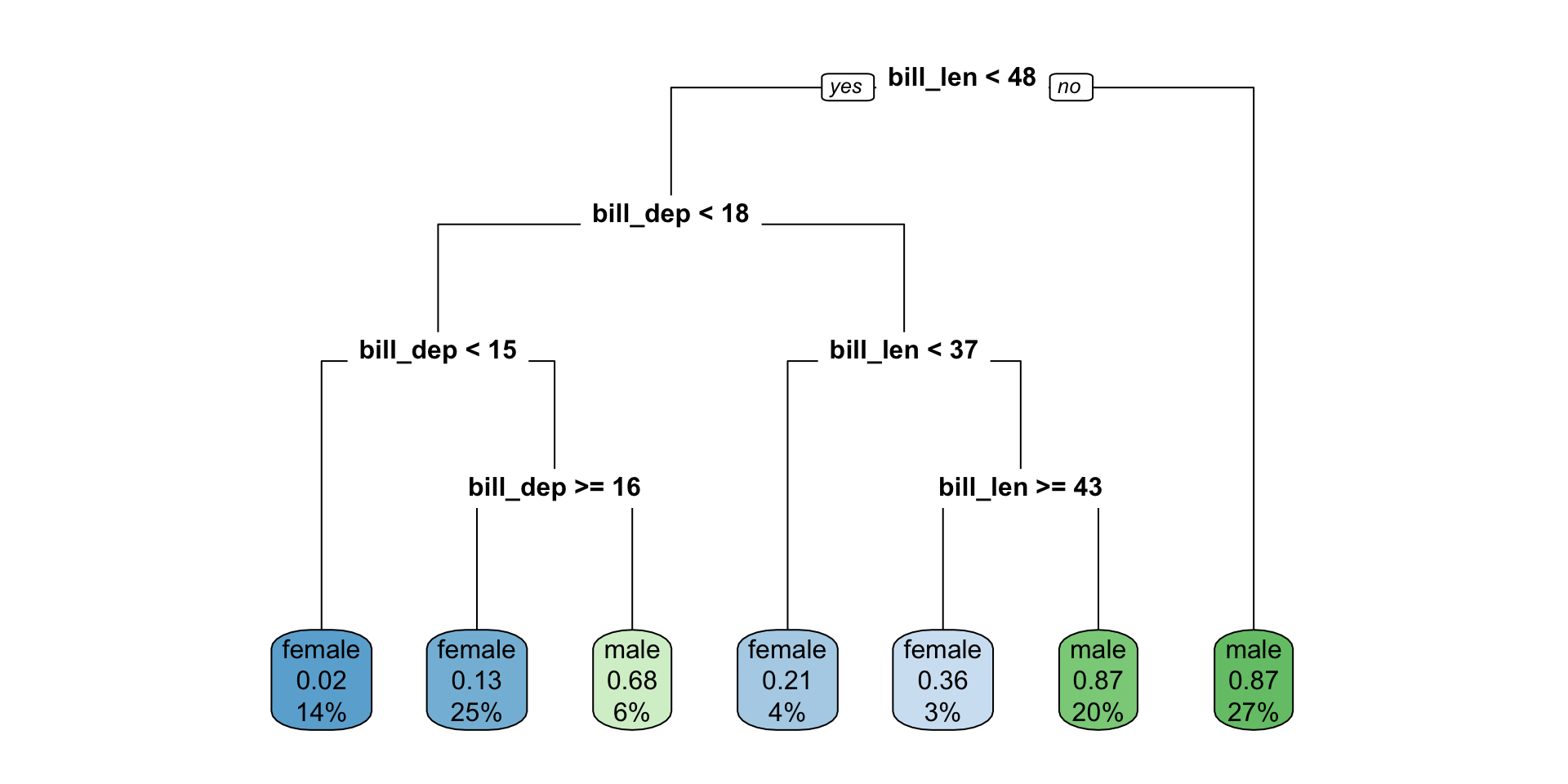
Classification tree with tidymodels
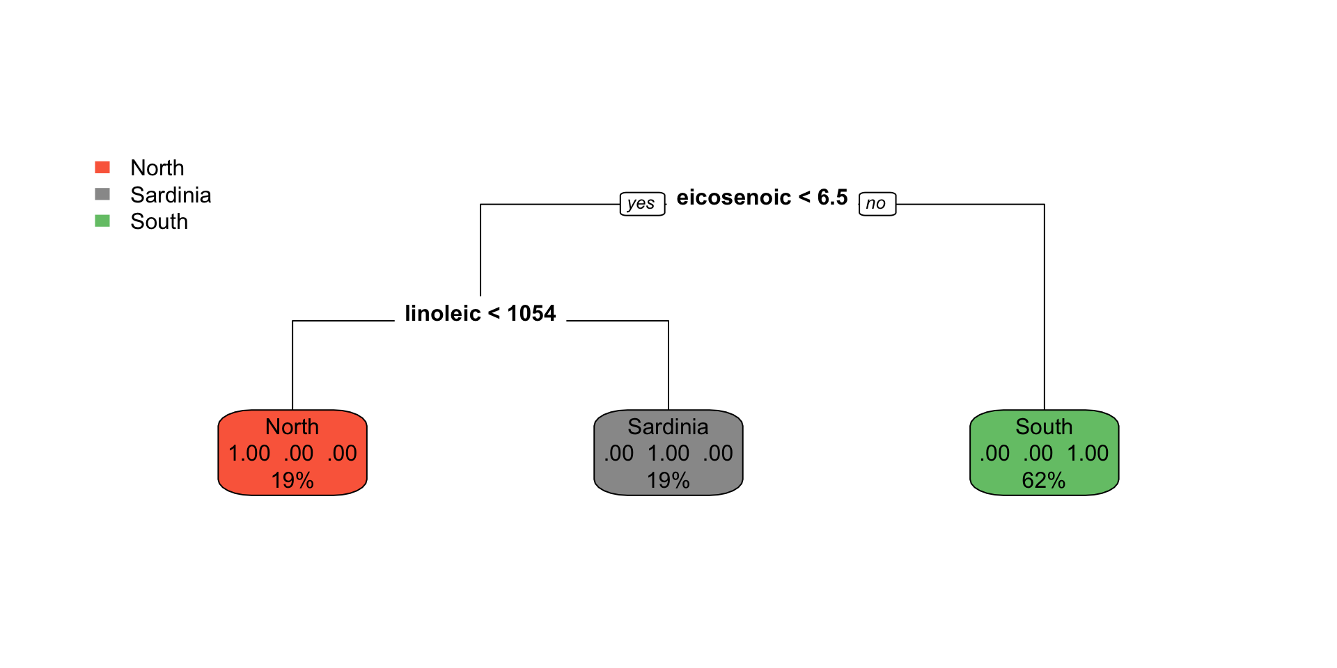
library (rpart.plot)|> extract_fit_engine () |> :: rpart.plot (type = 0 )
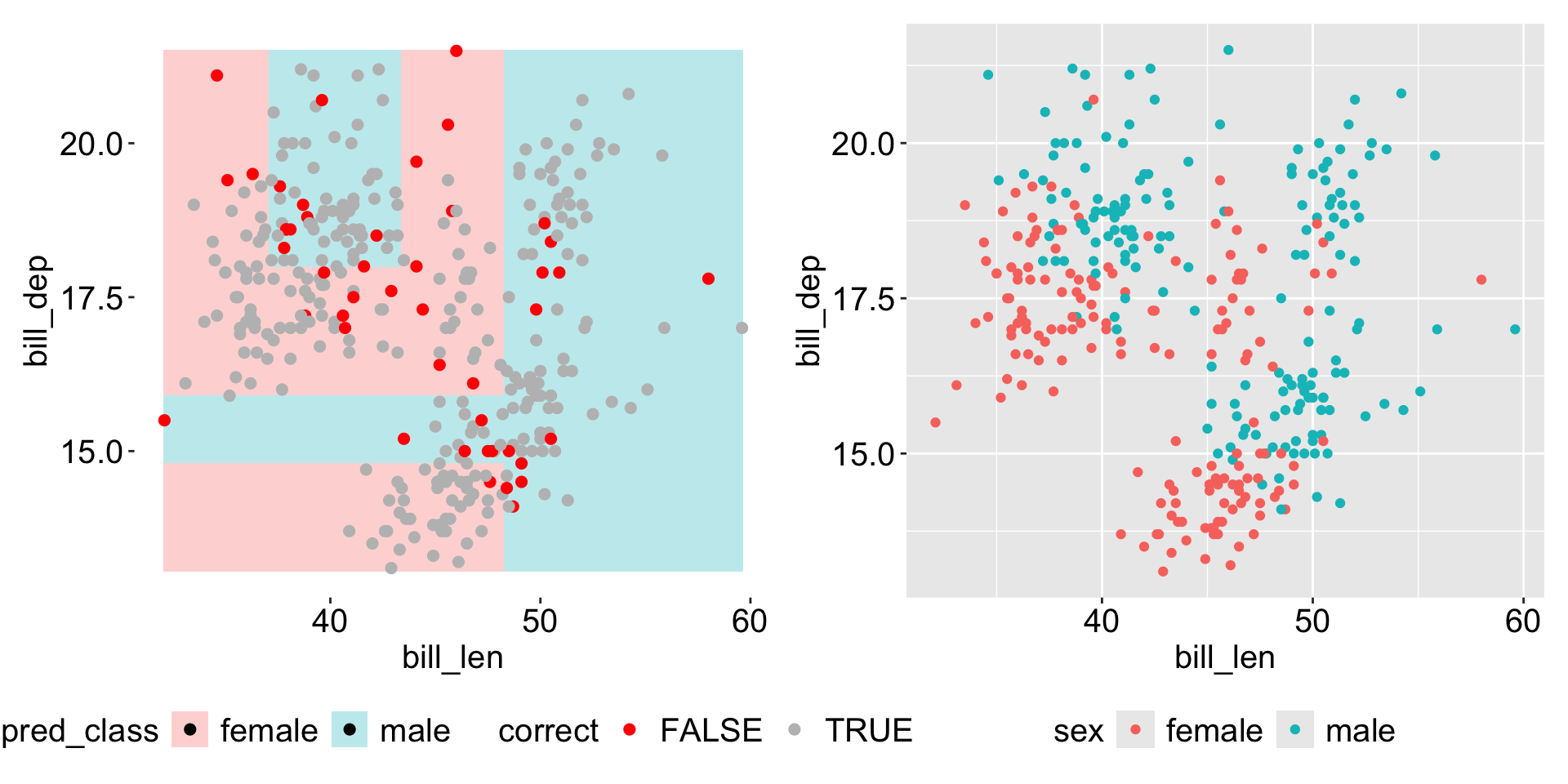
Visualize the space
More details on the tree parameters
By default, the Gini index is used for splitting the tree, to change to entropy, use
decision_tree (mode = "classification" ) |> set_engine ("rpart" , parms = list (split = "information" ))